Trading strategy for trading co-integrated stock pairs
The purpose of this article is to share the simplest strategy of statistical arbitrage based on trading in cointegrated pairs of stocks that were identified on the Moscow and New York stock exchanges.
If we take a pair of cointegrated shares, then we have the opportunity to hedge and build a market neutral strategy, when losses on one paper will be offset by profits on another. How does it look in practice?
Suppose we have a cointegrated pair of shares, X and Y , as well as the prices of these shares for a certain period of time 0,...,T . For example, let's take a couple of stocks with tickers (VSYDP, NKHP) from my previous article on cointegration . For her, we have price data for 215 trading days.
We will use the first half of the observations to determine the parameters of a trading strategy. Then, based on the parameters found, we take the second half of the observations and conduct backtests, that is, we will test whether such a strategy will bring us money.
')
For further discussion, I will need a spread of two stocks, st=yt− betaxt . In our example with a pair (VSYDP, NKHP) we already found a spread in the previous article on cointegration, so here I just duplicate the picture:
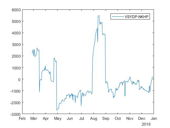
So, we all want to buy cheap and sell high. If the spread goes below zero, the stock Y (VSYDP) is cheaper than stock X (NKHP). Conversely, if the spread rises above zero, the stock Y more than share X (so or X cheaper compared to Y ).
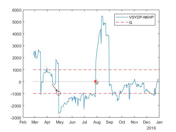
So, in essence, the trading strategy is to buy stock. Y and sell stock X in relation to 1: beta if the spread is slightly below zero (below the line G on the picture). When the spread returns to zero, we need to close the position by selling Y and buying X in the same ratio. In this case, we get profit size G :
Here it is important to understand that we must be able to sell stocks that we do not own — this is called short selling (short). It should also be noted that not all brokers include the possibility of a short sale in the standard package of services, so you may have to contact him in order to expand your investment opportunities.
In general, we make a portfolio that contains one long position (long) and one short position (short) if the spread crosses a certain line. G or goes for it in the opposite direction from zero. And we close all positions when the spread returns to zero.
The next question that arises is “how to find the meaning G "?
In addition to mathematics, I will immediately give here the implementation in the lab. The code below is a natural continuation of the code from the previous article on cointegration . We will need the first half of the observations t=0,...,T/2 which we will consider as "history".
First, find the average ratio Y and X for the first half of the observations.
For a pair of stocks with tickers (VSYDP, NKHP), the calculated value barr=$34.392 . Then we calculate the maximum absolute value of the spread for the first half of the observations:
For a pair of stocks with tickers (VSYDP, NKHP), the calculated value m=3204.4 . Now we can determine the value G by iteration: take a certain percentage of m and try to trade on the "history" at different values of this percentage, and then choose the value that will give the greatest profit. This will be the desired value for the line. G .
First we need to count the number of trades. First trade, let's label it t1 we do when we first stand in the position. In this case, we still do not make a profit:
Where st - spread. Further successful moments of the trades will be:
Then the profit will be calculated as (d−1) cdot2g where d - number of trades, g - some percent of m . If there were no trades, then the profit is zero. (d−1) cdot2g - this is the minimum profit, if you always trade one ratio Y and betaX .
The table below shows the percentages and outcomes for a pair of stocks with tickers (VSYDP, NKHP).
To determine the value G , we simply choose the value that gives the greatest profit, based on the "history".
However, although G=$2563. (at 80% of m ) gives the greatest profit, in practice we do not choose G more than 0,5m , due to the difficulties associated with further profit, so we take G=$1121. (at 35% of m ).
After determining G trading strategy is applied to the second half of the observations.
With G=$1121. profit is extracted 3 times. In other words, the difference moves 3 times from 0 to G and back. Please note that the implementation of such a strategy involves 6 trades, since in order to take a position and exit it, you need to make two trades.
The figure and the table below show all 6 trading points.
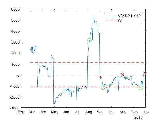
Profit earned here is at least 3G=3 cdot$1121.6=$3364. . It uses closing prices instead of intraday data, so we do not trade in points −G , 0 and G . As can be seen from the table, the yield for 107 trading days was 25.39%, excluding commissions, volume, etc. That is, this is approximately 60.74% per annum, according to very rough estimates.
Tests were also conducted for 58 pairs on the NYSE. There, except for zero profit, the approximate annual yield for this strategy ranged from 23.34% to 208% excluding commissions, volume, etc.
Instead of closing the position when the spread approaches zero, you can turn the position when the spread reaches G on the opposite side of zero. Suppose we sold 1Y and bought 35,6527X since the difference was greater G .
Now you can wait for the moment when the difference reaches −G to buy 2Y and sell 2 cdot35,6527X . As a result, we will stay with a portfolio from a long size position. 1Y and short size positions 35,6527X .
This strategy leads to one initial trade and one trade, which reverses the position. These trades are shown in the figure and in the table below.
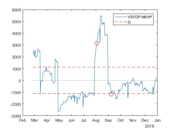
Please note that the profit from position reversal is 2G=2 cdot$1121.6=$2,243. therefore the total profit in this case is not less than 1 cdot2G=$2243. . As can be seen from the table, the yield for 107 trading days was 18.53% excluding commissions, volume, etc. That is, this is approximately 44.32% per annum, according to very rough estimates.
Tests were also conducted for 58 pairs on the NYSE. There, except for zero profit, the approximate annual yield for this strategy ranged from 17.63% to 201.53%, excluding commissions, volume, etc.
This change in the trading strategy reduces the number of trades by an average of 2 times. At the same time, trade costs are reduced. If the difference were moving up and down around 0, an alternative strategy would be more profitable. However, in the considered case, when the pair has a tendency to move between 0 and −G , the position in general never turns over, whereas the main strategy creates and eliminates the position again and again ... and makes money.
When trading co-integrated pairs, theoretically, it is possible to extract stable profits, in particular, using the methods described above in the form of two trading strategies. In the case of the considered pair of stocks (VSYDP, NKHP), the first method turned out to be more effective because of the tendency in their difference to fluctuate below zero.
The possibility of extracting stable profits when trading in cointegrated pairs looks optimistic, but it requires further analysis on demo accounts, which we will discuss next time.
Terry J. Wattsham, Kate Parramow. Quantitative methods in finance / Trans. from English by ed. Mr Efimova. - M .: Finance, UNITI, 1999. - 527 p.
This textbook was once taught for masters quantitative analysis at HSE. There is a section on cointegration.
UPD. Backtest results for 2017 on the Moscow Exchange
If we take a pair of cointegrated shares, then we have the opportunity to hedge and build a market neutral strategy, when losses on one paper will be offset by profits on another. How does it look in practice?
Trading strategy
Suppose we have a cointegrated pair of shares, X and Y , as well as the prices of these shares for a certain period of time 0,...,T . For example, let's take a couple of stocks with tickers (VSYDP, NKHP) from my previous article on cointegration . For her, we have price data for 215 trading days.
We will use the first half of the observations to determine the parameters of a trading strategy. Then, based on the parameters found, we take the second half of the observations and conduct backtests, that is, we will test whether such a strategy will bring us money.
')
For further discussion, I will need a spread of two stocks, st=yt− betaxt . In our example with a pair (VSYDP, NKHP) we already found a spread in the previous article on cointegration, so here I just duplicate the picture:
So, we all want to buy cheap and sell high. If the spread goes below zero, the stock Y (VSYDP) is cheaper than stock X (NKHP). Conversely, if the spread rises above zero, the stock Y more than share X (so or X cheaper compared to Y ).
So, in essence, the trading strategy is to buy stock. Y and sell stock X in relation to 1: beta if the spread is slightly below zero (below the line G on the picture). When the spread returns to zero, we need to close the position by selling Y and buying X in the same ratio. In this case, we get profit size G :
Here it is important to understand that we must be able to sell stocks that we do not own — this is called short selling (short). It should also be noted that not all brokers include the possibility of a short sale in the standard package of services, so you may have to contact him in order to expand your investment opportunities.
In general, we make a portfolio that contains one long position (long) and one short position (short) if the spread crosses a certain line. G or goes for it in the opposite direction from zero. And we close all positions when the spread returns to zero.
The next question that arises is “how to find the meaning G "?
How to find the value G
In addition to mathematics, I will immediately give here the implementation in the lab. The code below is a natural continuation of the code from the previous article on cointegration . We will need the first half of the observations t=0,...,T/2 which we will consider as "history".
T = length(testPrices); half = round(T/2); First, find the average ratio Y and X for the first half of the observations.
barr= frac1T/2+1 sumT/2t=0 fracytxt.
sumRatio = 0; for i = 1 : half sumRatio = sumRatio + testPrices(i,1) / testPrices(i,2); end r = sumRatio / half; For a pair of stocks with tickers (VSYDP, NKHP), the calculated value barr=$34.392 . Then we calculate the maximum absolute value of the spread for the first half of the observations:
m= maxt|yt− barrxt|,t=0,...,T/2.
clear absspread for i = 1 : half absspread(i,1) = abs(testPrices(i,1) - r * testPrices(i,2)); end m = max(absspread); For a pair of stocks with tickers (VSYDP, NKHP), the calculated value m=3204.4 . Now we can determine the value G by iteration: take a certain percentage of m and try to trade on the "history" at different values of this percentage, and then choose the value that will give the greatest profit. This will be the desired value for the line. G .
Enumerate different values G to find the best
First we need to count the number of trades. First trade, let's label it t1 we do when we first stand in the position. In this case, we still do not make a profit:
t1= mint:|st| geqg,
Where st - spread. Further successful moments of the trades will be:
- if a stn geqg : tn+1= mint:t>tn,st leq−g ;
- if a stn leq−g : tn+1= mint:t>tn,st geqg .
Then the profit will be calculated as (d−1) cdot2g where d - number of trades, g - some percent of m . If there were no trades, then the profit is zero. (d−1) cdot2g - this is the minimum profit, if you always trade one ratio Y and betaX .
clear profit for h = 1:10 g = 0.05 * h * m; profit(h,1) = 0.05 * h * 100; profit(h,2) = g; clear trade k = 1; for i = 1:half - 1 if abs(spread(i)) >= g trade(1,1) = i; trade(1,2) = spread(i); trade(1,3) = -1; trade(1,4) = beta; trade(1,5) = testPrices(i,1); trade(1,6) = testPrices(i,2); trade(1,7) = 0; startIndex = i; k = 2; break end end if k == 1 break end for i = startIndex:half - 1 if (trade(k-1,2) <= -g) && (spread(i) <= g) && (spread(i+1) >= g) trade(k,1) = i+1; trade(k,2) = spread(i+1); trade(k,3) = -1; trade(k,4) = beta; trade(k,5) = testPrices(i+1,1); trade(k,6) = testPrices(i+1,2); trade(k,7) = 0; k = k + 1; end if (trade(k-1,2) >= g) && (spread(i) > -g) && (spread(i+1) <= -g) trade(k,1) = i+1; trade(k,2) = spread(i+1); trade(k,3) = 1; trade(k,4) = -beta; trade(k,5) = testPrices(i+1,1); trade(k,6) = testPrices(i+1,2); trade(k,7) = 0; k = k + 1; end end if exist('trade', 'var') tradesNumber = size(trade,1); profit(h,3) = tradesNumber; profit(h,4) = (tradesNumber - 1) * 2 * g; else profit(h,3) = 0; profit(h,4) = 0; end end The table below shows the percentages and outcomes for a pair of stocks with tickers (VSYDP, NKHP).
| Percent | G | Trades | Profit |
|---|---|---|---|
| five | 160,2224 | 7 | 1922.7 |
| ten | 320,4449 | five | 2563.6 |
| 15 | 480,6673 | five | 3845.3 |
| 20 | 640,8898 | five | 5127.1 |
| 25 | 801,1122 | five | 6408.9 |
| thirty | 961,3347 | five | 7690.7 |
| 35 | 1121.6 | five | 8972,5 |
| 40 | 1281.8 | 3 | 5127.1 |
| 45 | 1442 | 3 | 5768 |
| 50 | 1602.2 | 3 | 6408.9 |
| 55 | 1762.4 | 3 | 7049,8 |
| 60 | 1922.7 | 3 | 7690.7 |
| 65 | 2082.9 | 3 | 8331,6 |
| 70 | 2243.1 | 3 | 8972,5 |
| 75 | 2403.3 | 3 | 9613.3 |
| 80 | 2563.6 | 3 | 10254 |
| 85 | 2723.8 | one | 0 |
| 90 | 2884 | 0 | 0 |
To determine the value G , we simply choose the value that gives the greatest profit, based on the "history".
[M, I] = max(profit(:,4)); bestG = profit(I,2); However, although G=$2563. (at 80% of m ) gives the greatest profit, in practice we do not choose G more than 0,5m , due to the difficulties associated with further profit, so we take G=$1121. (at 35% of m ).
Strategy testing
After determining G trading strategy is applied to the second half of the observations.
clear strategy for i = half + 1:T if abs(spread(i)) >= bestG strategy(1,1) = i; strategy(1,2) = spread(i); if spread(i) > 0 strategy(1,3) = -1; strategy(1,4) = beta; else strategy(1,3) = 1; strategy(1,4) = -beta; end strategy(1,5) = testPrices(i,1); strategy(1,6) = testPrices(i,2); strategy(1,7) = 0; startIndex = i; break end end if exist('strategy', 'var') k = 2; for i = startIndex:T-1 if (strategy(k-1,3) ~= 0) if (spread(i) >= 0) && (spread(i+1) <= 0) strategy(k,1) = i+1; strategy(k,2) = spread(i+1); strategy(k,3) = 0; strategy(k,4) = 0; strategy(k,5) = testPrices(i+1,1); strategy(k,6) = testPrices(i+1,2); strategy(k,7) = strategy(k-1,2) - spread(i+1); k = k + 1; end if (spread(i) <= 0) && (spread(i+1) >= 0) strategy(k,1) = i+1; strategy(k,2) = spread(i+1); strategy(k,3) = 0; strategy(k,4) = 0; strategy(k,5) = testPrices(i+1,1); strategy(k,6) = testPrices(i+1,2); strategy(k,7) = spread(i+1) - strategy(k-1,2); k = k + 1; end else if (spread(i) <= bestG) && (spread(i+1) >= bestG) strategy(k,1) = i+1; strategy(k,2) = spread(i+1); strategy(k,3) = -1; strategy(k,4) = beta; strategy(k,5) = testPrices(i+1,1); strategy(k,6) = testPrices(i+1,2); strategy(k,7) = 0; k = k + 1; end if (spread(i) >= -bestG) && (spread(i+1) <= -bestG) strategy(k,1) = i+1; strategy(k,2) = spread(i+1); strategy(k,3) = 1; strategy(k,4) = -beta; strategy(k,5) = testPrices(i+1,1); strategy(k,6) = testPrices(i+1,2); strategy(k,7) = 0; k = k + 1; end end end end if exist('strategy', 'var') totalProfit = sum(strategy(:,7)); else totalProfit = 0; end With G=$1121. profit is extracted 3 times. In other words, the difference moves 3 times from 0 to G and back. Please note that the implementation of such a strategy involves 6 trades, since in order to take a position and exit it, you need to make two trades.
The figure and the table below show all 6 trading points.
| Trade | t | st | Position (Y,X) | Price Y | Price X | Profit |
|---|---|---|---|---|---|---|
| one | 108 | 3145.9 | (-1; +35.6527) | 13200 | 282 | - |
| 2 | 128 | -211,447 | Liquidation | 9700 | 278 | 3357.4 |
| 3 | 134 | -1161.9 | (+1; -35.6527) | 8500 | 271 | - |
| four | 171 | 14,6605 | Liquidation | 8500 | 238 | 1176.5 |
| five | 205 | -1184,5 | (+1; -35.6527) | 7800 | 252 | - |
| 6 | 212 | 185,1035 | Liquidation | 8100 | 222 | 1369.6 |
| Total | 5903,5 | |||||
Profit earned here is at least 3G=3 cdot$1121.6=$3364. . It uses closing prices instead of intraday data, so we do not trade in points −G , 0 and G . As can be seen from the table, the yield for 107 trading days was 25.39%, excluding commissions, volume, etc. That is, this is approximately 60.74% per annum, according to very rough estimates.
Tests were also conducted for 58 pairs on the NYSE. There, except for zero profit, the approximate annual yield for this strategy ranged from 23.34% to 208% excluding commissions, volume, etc.
Testing an alternative strategy
Instead of closing the position when the spread approaches zero, you can turn the position when the spread reaches G on the opposite side of zero. Suppose we sold 1Y and bought 35,6527X since the difference was greater G .
Now you can wait for the moment when the difference reaches −G to buy 2Y and sell 2 cdot35,6527X . As a result, we will stay with a portfolio from a long size position. 1Y and short size positions 35,6527X .
clear strategyAlt for i = half + 1:T if abs(spread(i)) >= bestG strategyAlt(1,1) = i; strategyAlt(1,2) = spread(i); if spread(i) > 0 strategyAlt(1,3) = -1; strategyAlt(1,4) = beta; else strategyAlt(1,3) = 1; strategyAlt(1,4) = -beta; end strategyAlt(1,5) = testPrices(i,1); strategyAlt(1,6) = testPrices(i,2); strategyAlt(1,7) = 0; startIndex = i; break end end if exist('strategyAlt', 'var') d = 2; for i = startIndex:T-1 if (strategyAlt(d-1,2) >= bestG) && (spread(i) >= -bestG) && (spread(i+1) <= -bestG) strategyAlt(d,1) = i+1; strategyAlt(d,2) = spread(i+1); strategyAlt(d,3) = 1; strategyAlt(d,4) = -beta; strategyAlt(d,5) = testPrices(i+1,1); strategyAlt(d,6) = testPrices(i+1,2); strategyAlt(d,7) = strategyAlt(d-1,2) - spread(i+1); d = d + 1; end if (strategyAlt(d-1,2) <= -bestG) && (spread(i) <= bestG) && (spread(i+1) >= bestG) strategyAlt(d,1) = i+1; strategyAlt(d,2) = spread(i+1); strategyAlt(d,3) = -1; strategyAlt(d,4) = beta; strategyAlt(d,5) = testPrices(i+1,1); strategyAlt(d,6) = testPrices(i+1,2); strategyAlt(d,7) = spread(i+1) - strategyAlt(d-1,2); d = d + 1; end end end if exist('strategyAlt', 'var') totalAltProfit = sum(strategyAlt(:,7)); else totalAltProfit = 0; end This strategy leads to one initial trade and one trade, which reverses the position. These trades are shown in the figure and in the table below.
| Trade | t | st | Position (Y,X) | Price Y | Price X | Profit |
|---|---|---|---|---|---|---|
| one | 108 | 3145.9 | (-1; +35.6527) | 13200 | 282 | - |
| 2 | 134 | -1161.9 | (+1; -35.6527) | 8500 | 271 | 4307.8 |
| Total | 4307.8 | |||||
Please note that the profit from position reversal is 2G=2 cdot$1121.6=$2,243. therefore the total profit in this case is not less than 1 cdot2G=$2243. . As can be seen from the table, the yield for 107 trading days was 18.53% excluding commissions, volume, etc. That is, this is approximately 44.32% per annum, according to very rough estimates.
Tests were also conducted for 58 pairs on the NYSE. There, except for zero profit, the approximate annual yield for this strategy ranged from 17.63% to 201.53%, excluding commissions, volume, etc.
This change in the trading strategy reduces the number of trades by an average of 2 times. At the same time, trade costs are reduced. If the difference were moving up and down around 0, an alternative strategy would be more profitable. However, in the considered case, when the pair has a tendency to move between 0 and −G , the position in general never turns over, whereas the main strategy creates and eliminates the position again and again ... and makes money.
findings
When trading co-integrated pairs, theoretically, it is possible to extract stable profits, in particular, using the methods described above in the form of two trading strategies. In the case of the considered pair of stocks (VSYDP, NKHP), the first method turned out to be more effective because of the tendency in their difference to fluctuate below zero.
The possibility of extracting stable profits when trading in cointegrated pairs looks optimistic, but it requires further analysis on demo accounts, which we will discuss next time.
What to read on the topic
Terry J. Wattsham, Kate Parramow. Quantitative methods in finance / Trans. from English by ed. Mr Efimova. - M .: Finance, UNITI, 1999. - 527 p.
This textbook was once taught for masters quantitative analysis at HSE. There is a section on cointegration.
UPD. Backtest results for 2017 on the Moscow Exchange
Source: https://habr.com/ru/post/344674/
All Articles