The history of victory in the international competition for the recognition of documents of the SmartEngines company
Hi, Habr! Today we will talk about how our Smart Engines team managed to win the international binarization of documents DIBCO17 held at the ICDAR conference. This competition is held regularly and already has a solid history (it has been held for 9 years), during which many incredibly interesting and insane (in a good way) binarization algorithms were proposed. Despite the fact that we do not use such algorithms in our document recognition projects using mobile devices, the team seemed to have something to offer the world community, and this year we made the decision to participate in the competition for the first time.

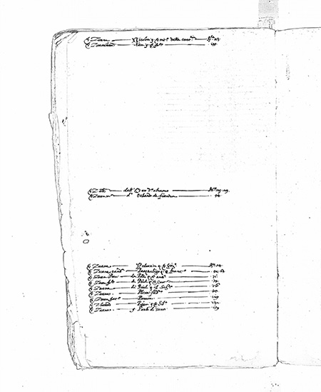
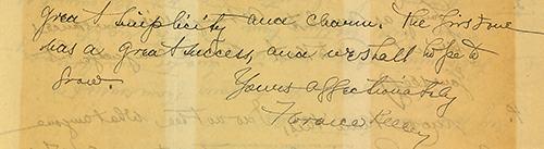
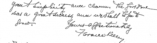
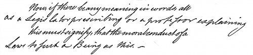
To begin with, let us briefly explain what its essence is: given a lot of color images of documents S prepared by the organizers (an example of one of these images is shown in the figure to the left) and a lot of binary images I (ground truth, the expected result for an example is shown in the figure to the right) It is required to construct an algorithm A that translates the source images from S into two-level black-and-white a ( A ) (i.e., solve the problem of classifying each pixel as belonging to an object or background) so that these resulting images are as close as possible to corresponding to the ideal of i . The set of metrics by which this proximity is evaluated is, of course, recorded in the conditions of competition. The peculiarity of this competition is that no test image is provided in advance to the contestants, data from past contests are available for setup and preparation. At the same time, the new data each time contains its own “zest”, which distinguishes them from previous contests (for example, the presence of thin “watercolor” text styles or characters that appear translucent on the opposite side) and present new challenges for participants. The competition regularly gathers about two to three dozen participants from around the world. The following is a description of our competitive decision.


Solution scheme
The first step was collected data from all previous contests. In total, we managed to upload 65 images of handwritten documents and 21 images printed. Obviously, in order to achieve high results, it was necessary to look at the problem with a wider view, therefore, in addition to analyzing the images from the organizers, we searched for open data with archival printed and handwritten documents. The organizers did not prohibit the use of third-party datasets. Several thousand images were successfully found that, by their nature, fit the conditions of the competition (data from various thematic competitions organized by ICDAR, the READ project, and others). After studying and classifying these documents, it became clear which classes of problems we could encounter in principle, and which of them remained until now ignored by the organizers of the competition. For example, in none of the previous competitions the documents contained no elements of the graphic, although the tables are often found in the archives.
In preparation for the competition, we walked in parallel in several ways. In addition to the classical algorithmic approaches that we have studied well before, it was decided to try out machine learning methods for pixel classification of object-background, despite the very small amount of data originally provided. Since in the end it was precisely this approach that turned out to be the most effective, we will tell about it.
Selection of network architecture
As the initial version, the neural network of the U-net architecture was chosen. Such architecture has proven itself in solving segmentation problems in various competitions (for example, 1 , 2 , 3 ). An important consideration was the fact that a large class of well-known binarization algorithms is explicitly expressed in such an architecture or a similar architecture (as an example, we can take a modification of the Niblack algorithm with the replacement of the standard deviation by the mean deviation modulus, in this case the network is especially simple).
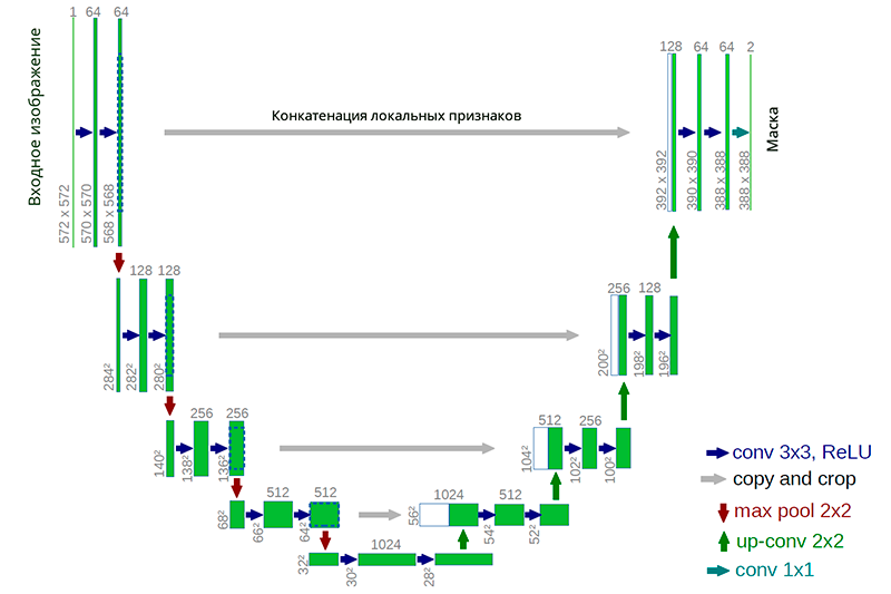
An example of a neural network U-net architecture
The advantage of this architecture is that for network training you can create a sufficient amount of training data from a small number of source images. At the same time, the network has a relatively small number of weights due to its convolutional architecture. But there are some nuances. In particular, the artificial neural network used, strictly speaking, does not solve the problem of binarization: it assigns to each pixel of the original image a certain number from 0 to 1, which characterizes the degree of belonging of this pixel to one of the classes (meaningful filling or background) and still convert to final binary answer.
As a training sample, 80% of the original images were taken. The remaining 20% of the images were allocated for validation and testing. Images from color were converted to grayscale to avoid retraining, after which they were all cut into non-overlapping windows of 128x128 pixels. The optimal window size was chosen empirically (windows from 16x16 to 512x512 were tried). Initially, no augmentation methods were used, and thus, from a hundred of initial images, about 70 thousand windows were obtained, which were fed to the input of the neural network. Each such window of the image was assigned a binary mask cut from the markup.

Window samples
The parameters of the neural network, the learning process and data augmentation took place in manual mode, since each experiment (data augmentation, training / further training of the network, validation and testing of the solution) took several hours, and the principle of “looking at carefully and understanding what is happening” in our opinion is preferable to running hyperopt for a week. Adam was chosen as the method of stochastic optimization. Cross-entropy was used as a metric for the loss function.
Primary experiments
Already the first experiments showed that such an approach allows achieving higher quality than the simplest non-learning methods (such as Father or Niblack). The neural network was well trained and the learning process quickly converged to an acceptable minimum. The following are some examples of animation of the network learning process. The first two images are taken from the original datasets, the third is found in one of the archives.
Each of the animations was obtained as follows: in the process of learning the neural network, as the quality improves, the same source image is run through the network. The results of the network are glued together in one gif animation.

Original handwriting image with complex background

The result of binarization as learning network
The complexity of the binarization of the above example is to distinguish the heterogeneous background from the ornate handwriting. Part of the letters is blurred, text appears on the other page, blots. The one who wrote this manuscript is clearly not the most accurate person of his time =).

Original printed text image with previous page's treads

The result of binarization as learning network
In this example, in addition to the non-uniform background, there is also text that appeared from the previous page. The difference by which it can be determined that the shrunk text needs to be classified as "background" is the wrong "mirror" character.


Image with a table and the result of its binarization in the process of network learning
After each experiment, we additionally evaluated the relevance of the obtained model on a set of selected data from open archives and on various types of printed documents and questionnaires. It was noted that when applying a network to examples from this data, the result of the algorithm was often unsatisfactory. It was decided to add such images to the training set. The most problematic cases were the edges of the pages of documents and their marking lines. A total of 5 additional images were selected containing the objects of interest. Primary binarization was performed using the existing network version, after which the pixels were verified by an expert, and the resulting images were added to the training sample.

In the example above, you can see that the network highlights the edges of the pages, which is an error


Here, in addition to network errors at the edges of the pages, there is still a very "uncertain" selection of the lines of the table and the text inside it.
Used augmentation techniques and how they help
In the process of network training and error analysis, data augmentation methods were used to improve the quality. The following types of distortion were used: reflections of images relative to the axes, brightness, projective, noise (Gaussian noise, salt-pepper), elastic transformations, like such ones, were tried out, a variation of the image scale. The use of each of them is due to the specifics of the problem, the observed errors in the network, as well as common practices.
An example of a combination of several augmentation methods that are applied “on the fly” in the network learning process
Since when generating data with all the various distortions and their combinations, the number of examples grows rapidly, augmentation is applied on the fly, in which the sample is blown up just before the examples for training are given. Schematically, this can be represented as:
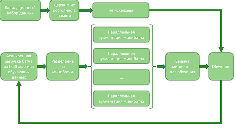
Diagram showing the process of blowing up data on the fly and issuing for training
This approach allows you to optimize the process of data swelling and network training, because:
- the number of accesses to the disk array decreases and it occurs sequentially, which makes it possible to speed up data loading many times.
- parallel data augmentation in mini-batches occurs independently and efficiently uses all the cores of the machine. Some of the most resource-intensive operations can be rewritten using theano / tensorflow and calculated on the 2nd gpu.
- Periodically, individual mini-batches are saved to disk, which allows checking the learning process and data blowing up.
- Most of the memory remains empty, since at the same time it stores about 20% of all data (validation set and current batch). This allows
shake 5 experiments at onceEfficient use of server computing resources.
In general, I would like to note the importance of proper augmentation - thanks to this technique, you can train a more complex and intelligent network on the one hand, and on the other, avoid retraining and be sure that the quality of network operation on a test sample is no worse than during training and validation. Some experts, for unknown reasons, neglect the work with data and are looking for a way to improve the system only by changing the architecture of networks. From our point of view , working with data is no less, and more often, more important than a thoughtful selection of network architecture parameters.
Quality improvement
The process of improving the quality of the decision took place iteratively. Most of the work went in three directions:
- Analysis of network errors and work with data.
- Refinement of network architecture, setting up hyperparameters of layers and regularization mechanisms.
- Construction of the ensemble on the basis of neural network and conventional methods.
Work with the data occurred in the following cycles:
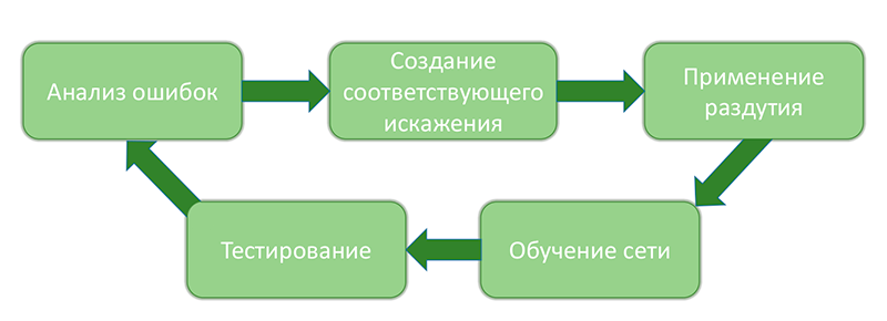
The process of analyzing system errors to eliminate them
The work with the data can be described in detail as follows: after each significant stage of the system change (with quality improvement, as we hoped each time), various metrics and statistics were calculated by cross-validation. About 2000 “windows” (but not more than 50 windows from one image) were written, on which the error reached the maximum value according to the quadratic metric and the images from which these windows were cut out. Then the analysis of these images and their classification by the type of error was carried out. The result looked like this:
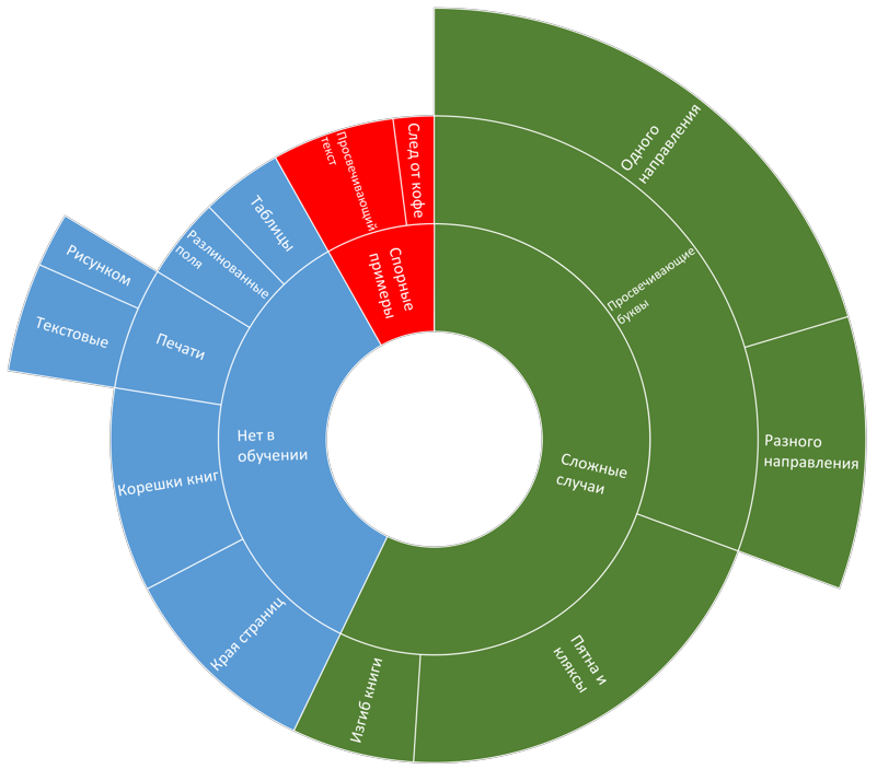
Sample Error Distribution Diagram
Next, select the most common type of error. A distortion is created that mimics images with this type of error. It is checked that the current version of the system is really wrong on the distorted image and the error occurs due to the added distortion. Then, the created augmentation procedure is added to the set of existing ones and is used in the learning process. After learning a new network and updating the system trim parameters, a new analysis and classification of errors occurs. As the final stage of the cycle - we check that the quality grows and the number of errors of a particular type has greatly decreased. Naturally, a very “idealistic” course of events is described here =). For example, for some types of errors, it is extremely difficult to create suitable distortions or when adding distorted images one type of errors may disappear and the other three may appear. Nevertheless, this methodology allows to level 80% of errors that occur at different stages of the system construction.
Example: in some images there is noise from a heterogeneous background, blots and, in particular, parchment grit. Errors that appear in such examples can be suppressed by additional noise in the original image.

An example of imitation of “granular parchment” using distortion
The process of optimization of the neural network architecture and layer hyperparameters was carried out in several directions:
- Variation of the current network architecture in depth / number of layers / number of filters, etc.
- Checking other architectures to solve our problem (VGG, Resnet, etc.). To test the possibility of using already trained neural networks, the networks of VGG and Resnet architectures were investigated. Two approaches were used:
- From the outputs of the different layers of each network, the vector signs were written off, which were used as the input of a fully connected neural network trained to solve the classification problem. In this case, only the “final” fully connected neural network was trained, and the networks supplying the signs remained unchanged. To reduce the dimension of the input space of a fully connected network, singular decomposition was used.
- The second approach was that we replaced the last N layers of one of the networks (for example, VGG) with fully connected ones and retrained the entire network. Those. just used ready weights as the initial initialization.
In general, it must be said that both approaches gave some results, but in terms of quality and reliability they were inferior to the U-net training approach “from scratch”.
Process ensembling
The next step in creating the final solution is to build an ensemble from several solutions. To build the ensemble, we used 3 U-net networks, different architectures, trained on different data sets, and one non-learning binarization method, which was used only at the edges of the image (for clipping pages edges).
We tried to build an ensemble in two different ways:
- Averaging the answers.
- Weighted sum of responses. The contribution to the final answer was determined by the quality of work on the validation sample.
In the process of working on the ensemble, we were able to achieve improved quality compared to a single U-net network. However, the improvement was very insignificant, and the work time of the ensemble consisting of several networks was extremely great. Even despite the fact that in this competition there was no limit on the running time of the algorithm, the conscience did not allow us to commit such a decision.
The choice of the final decision
As we move to the final version of the algorithm, each of the stages (adding additional delimited data, structure variation, blow-up, etc.) was subjected to a process of cross-validation, in order to understand whether we are doing everything correctly.
The final decision was chosen based on these statistics. They were exactly one U-net network, well trained with the application of everything described above + clipping on the threshold.
One possible way to provide a solution to the organizers was to create a docker container with a solution image. Unfortunately, it was not possible to use the container with gpu support (the organizers' requirement), and the final calculation was only for cpu. In this regard, some clever tricks were also removed, which allows a little higher quality. For example, initially, each image we chased through the grid several times:
- normal image
- mirrored
- upside down
- slightly reduced
- slightly enlarged
Then the results were averaged.
As the subsequent results showed, even without such tricks, the quality of the network’s operation was enough to take first place on both test datasets =)
results
This year, 18 teams from around the world took part in the competition. There were participants from the USA, China, India, Europe, countries of the Middle East and even from Australia. A variety of solutions were proposed using neural network models, modifications of classical adaptive methods, game theory, and combinations of various approaches. At the same time, a large variability was observed in the types of architectures used by neural networks. Both fully connected, convolutional, and recurrent variants with LSTM layers were used. As a preprocessing stage, for example, filtering and morphology were used. In the original article, they briefly described all the methods used by the participants - often they are so different that one can only wonder how they show a similar result.
Our solution managed to take the first place both on handwritten documents and on printed documents. The following are the final results of the measurement solutions. The description of the metrics can be found in the works of the organizers of the competition published in previous years. We briefly describe only the top 5 results, the rest can be read in the original article (a link to it should soon appear on the official website of the competition ). As a guideline, the organizers provide measurements for the classic Otsu classical zero-parametric global method and Sauvola's local low-parametric authorship (unfortunately, the exact values of the tuning coefficients are unknown).
| No | Brief description of the method | Score | FM | Fps | PSNR | DRD |
|---|---|---|---|---|---|---|
| one | Our method (U-net network) | 309 | 91.01 | 92.86 | 18.28 | 3.40 |
| 2 | FCN (VGG similar architecture) + postfiltering | 455 | 89.67 | 91.03 | 17.58 | 4.35 |
| 3 | Ensemble of 3 DSN, with 3-level output, working on patches of various scales | 481 | 89.42 | 91.52 | 17.61 | 3.56 |
| four | Ensemble of 5 FCN - entrance: patches of different scales + binarized by howe method + RD signs. | 529 | 86.05 | 90.25 | 17.53 | 4.52 |
| five | Similar to the previous method, but added CRF construction processing | 566 | 83.76 | 90.35 | 17.07 | 4.33 |
| ... | ... | ... | ... | ... | ... | ... |
| 7 | Morphology + Howe + post processing | 635 | 89.17 | 89.88 | 17.85 | 5.66 |
| Otsu | 77.73 | 77.89 | 13.85 | 15.5 | ||
| Sauvola | 77.11 | 84.1 | 14.25 | 8.85 |
The best method, not using any way neural nets, took the 7th place.
The following demonstrates the operation of our algorithm on a number of test images.


Well, the testimony that we were presented at the ICDAR 2017 conference in Japan:

')
Source: https://habr.com/ru/post/344550/
All Articles