Offtop

The title of the article did not fit - these results are considered as such according to the version of Graph500 rating. I would also like to thank IBM and RSC companies for providing resources for conducting experimental launches during the study.

Introduction

Wide Search (BFS) is one of the main graph traversal algorithms and the base for many higher-level graph analysis algorithms. A wide search on graphs is a task with irregular memory access and irregular data dependence, which greatly complicates its parallelization on all existing architectures. The article will discuss the implementation of a wider search algorithm (the main test of the Graph500 rating) for processing large graphs on various architectures: Intel x86, IBM Power8 +, Intel KNL and NVidia GPU. The features of the implementation of the algorithm on shared memory will be described, as well as graph transformations, which allow achieving record-high performance and energy efficiency indicators for this algorithm among all single-site Graph500 and GreenGraph500 rating systems.

Recently, graphic accelerators (GPU) in non-graphical calculations play an increasing role. The need for their use is due to their relatively high performance and lower cost. As you know, on the GPU and central processing units (CPUs), problems are well solved on structural, regular grids, where parallelism is somehow easily distinguished. But there are tasks that require high power and use unstructured grids or data. Examples of such tasks are: Single Shortest Source Path problem ( SSSP ) - the task of finding the shortest paths from a given vertex to all others in a weighted graph, the Breadth First Search (BFS [1]) problem - the task of finding a width in an undirected graph, Minimum Spanning Tree (MST, for example, foreign and my implementation) - the task of finding strongly related components and others.

These tasks are basic in a number of algorithms on graphs. Currently, the BFS and SSSP algorithms are used to rank computers in the Graph500 and GreenGraph500 ratings. The BFS algorithm (breadth-first search or search wide) is one of the most important graph analysis algorithms. It is used to obtain some properties of links between nodes in a given graph. BFS is mainly used as a link, for example, in such algorithms as finding connected components [2], finding the maximum flow [3], finding central components (between centrality) [4, 5], clustering [6], and many others.

The BFS algorithm has a linear computational complexity O (n + m), where n is the number of vertices and m is the number of edges of the graph. This computational complexity is optimal for consistent implementation. But this estimate of computational complexity is not applicable for parallel implementation, since the sequential implementation (for example, using the Dijkstra algorithm ) has data dependencies, which prevents its parallelization. Also, the performance of this algorithm is limited by the memory performance of a particular architecture. Therefore, the most important are the optimization aimed at improving the work with memory of all levels.

Review of existing solutions and Graph500 rating

Graph500 and GreenGraph500

The Graph500 rating was created as an alternative to the Top500 rating. This rating is used to rank computers in applications that use irregular memory access, as opposed to the latter. For the tested application in the Graph500 rating, the memory and communication network bandwidth play the most important role. The GreenGraph500 rating is an alternative to the Green500 rating and is used in addition to Graph500.

Graph500 uses the metric - the number of processed edges of the graph per second (TEPS - traversed edges per second), while GreenGraph500 uses the metric - the number of processed edges of the graph per second per watt. Thus, the first rating ranks the computers according to the speed of computation, and the second according to the energy efficiency. These ratings are updated every six months.

Existing solutions

The width search algorithm was invented more than 50 years ago. And research is still being conducted for effective parallel implementation on various devices. This algorithm shows how well the work with memory and communication environment of calculators is organized. There are a lot of works on parallelization of this algorithm on x86 systems [7-11] and on the GPU [12-13]. Also, detailed results of the implementation of the implemented algorithms can be seen in the ratings of Green500 and GreenGraph500. Unfortunately, the algorithms of many effective implementations are not published in foreign sources.

If you select only single-node systems in the Graph500 rating, then we will get the following some data, which are presented in the table below. The results described in this paper are marked in bold. The table included graphs with more than 2 ²⁵ vertices. From the data obtained it can be seen that currently there is no more efficient implementation using only one node than the one proposed in this article. A more detailed analysis is presented in the Analysis section of the results .

Position	System	Size 2 n	GTEPS	Watt
50	GPU NVidia Tesla P100	26	204	175
67	NVidia GTX Titan GPU	25	114	212
76	4x Intel Xeon E7-4890 v2	32	55.9	1153
86	GPU NVidia Tesla P100	thirty	41.7	235
103	NVidia GTX Titan GPU	25	17.2	233.8
104	Intel Xeon E5 2699 v3	thirty	16.3	145
106	4x AMD Radeon R9 Nano GPUs	25	15.8
112	IBM POWER8 +	thirty	13.2	200

Graph storage format

To evaluate the performance of the BFS algorithm, undirected RMAT graphs are used . RMAT graphs model real graphs from social networks and the Internet well. In this case, RMAT graphs are considered with an average degree of connectivity of a vertex 16, and the number of vertices is a power of two. In such a RMAT graph, there is one large connected component and a number of small connected components or hanging vertices. The strong connectivity of the components does not allow in any way to divide the graph into such subgraphs that would fit in the cache memory.

To build the graph, a generator is used which is provided by the developers of the Graph500 rating. This generator creates an undirected graph in the RMAT format, with the output data presented as a set of graph edges. Such a format is not very convenient for an efficient parallel implementation of graph algorithms, since it is necessary to have aggregated information for each vertex, namely, which vertices are neighbors for a given one. A convenient format for this view is called CSR (Compressed Sparse Rows).

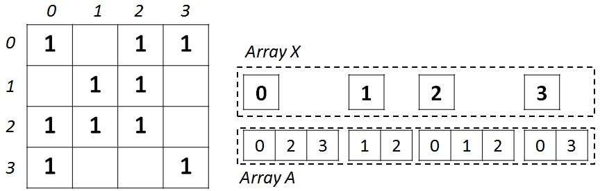
This format is widely used to store sparse matrices and graphs. For an undirected graph with N vertices and M edges, two arrays are needed: X (an array of pointers to adjacent vertices) and A (an array of a list of adjacent vertices). Array X of size N + 1, and array A is 2 * M, since in an undirected graph for any pair of vertices it is necessary to store forward and backward arcs. The array X stores the beginning and the end of the list of neighbors located in array A, that is, the entire list of neighbors of the vertex J is in array A from the index X [J] to X [J + 1], not including it. For illustration, the figure below shows a graph of 4 vertices on the left, written using an adjacency matrix, and on the right, in CSR format.

After converting the graph to the CSR format, it is necessary to do some more work on the input graph to improve the efficiency of the cache and memory of computing devices. After performing the transformations described below, the graph remains in the same CSR format, but acquires some properties related to the transformations performed.

The transformations introduced allow constructing the graph in the optimal form for most of the algorithms for traversing the graph in the CSR format. Adding a new vertex to the graph will not re-execute all transformations; it is enough to follow the rules entered and add a vertex so that the general order of the vertices is not violated.

Local Sorting Vertex List

For each vertex, we will sort by ascending its neighbor list. As a key for sorting, we will use the number of neighbors for each vertex to be sorted. After performing this sorting, performing a traversal of the list of neighbors at each vertex, we will process first the heaviest vertices — vertices that have a large number of neighbors. This sorting can be performed independently for each vertex and in parallel. After performing this sorting, the number of vertices of the graph in memory does not change.

Global vertex list sorting

For a list of all the vertices of the graph, sort by ascending. As the key, we will use the number of neighbors for each of the vertices. Unlike local sorting, this sorting requires renumbering the received vertices, since the position of the vertex in the list changes. The sorting procedure has O (N * log (N)) complexity and is performed sequentially, and the vertex renumbering procedure can be performed in parallel and is comparable in speed to the copying time of one memory section to another.

Renumbering all vertices of the graph

Enumerate the vertices of the graph in such a way that the most connected vertices have the closest numbers. This procedure is arranged as follows. First the first vertex from the list is rendered for renumbering. It gets the number 0. Then all adjacent vertices with the vertex under consideration are added to the queue for renumbering. The next vertex from the renumbering list gets the number 1 and so on. As a result of this operation, in each connected component, the difference between the maximum and minimum vertex numbers will be the smallest, which will make the best use of the small cache of computing devices.

Algorithm implementation

The width search algorithm in an undirected graph is organized as follows. At the entrance is the initial for the previously undefined vertex in the graph (root vertex for the search). The algorithm must determine at what level, starting from the root vertex, each of the vertices in the graph is located. The level is understood as the minimum number of edges that must be overcome in order to get from the root vertex to the vertex other than the root. Also for each of the vertices, except the root, it is necessary to determine the vertex of the parent. Since one vertex can have several parent vertices, any of them is taken as the answer.

The wide search algorithm has several implementations. The most effective implementation is an iterative traversal of a graph with level synchronization. Each step is an iteration of the algorithm in which information from level J is transferred to level J + 1. The pseudocode of the sequential algorithm is presented by reference .

A parallel implementation is based on a hybrid algorithm consisting of top-down (TD) and bottom-up (BU) procedures, which was proposed by the author of this article [11]. The essence of this algorithm is as follows. The TD procedure allows you to bypass the vertices of the graph in a direct order, that is, going through the vertices, we consider the connection $$$V1 \ Rightarrow V2$as a parent-child. The second BU procedure allows you to bypass the vertices in the reverse order, that is, going through the vertices, we consider the connection $$$V1 \ Rightarrow V2$as a descendant parent.

Consider a sequential implementation of a hybrid TD-BU algorithm, the pseudo-code of which is shown below. To process the vertex graph, we need to create two additional queue arrays that will contain a set of vertices at the current level - Q _curr , and a set of vertices at the next level - Q _next . To perform faster checks for the existence of a vertex in the queue, you must enter an array of visited vertices. But since, as a result of the algorithm, we need to get information about the level at which each of the vertices is located, this array can also be used as an indicator of visited and marked vertices.

Sequential BFS hybrid algorithm:

void bfs_hybrid(G, N, M, Vstart) { Levels <- (-1); Parents <- (N + 1); Qcurr+=Vstart; CountQ=lvl=1; while (CountQ) { CountQ = 0; vis = 0; inLvl = 0; if (state == TD) foreach Vi in Qcurr foreach Vk in G.Edges(Vi) inLvl++; if (Levels[Vk] == -1) Qnext += Vk; Levels[Vk] = lvl; Parents[Vk] = Vi; vis++; else if (state == BU) foreach Vi in G if (Levels[Vi] == -1) foreach Vk in G.Edges(Vi) inLvl++; if (Levels[Vk] == lvl - 1) Qnext += Vi; Levels[Vi] = lvl; Parents[Vi] = Vk; vis++; break; change_state(Qcurr, Qnext, vis, inLvl, G); Qcurr <- Qnext; CountQ = Qnext.size(); } } 

The main loop of the algorithm consists of the sequential processing of each vertex in the Q _curr queue. If there are no more vertices left in the Q _curr queue, the algorithm stops and the answer is received.

At the very beginning of the algorithm, the TD procedure starts working, since the queue contains only one vertex. In the TD procedure, for each vertex V _i from the Q _curr queue, we look at the list of neighbors with this vertex V _k and add to the Q _next queue those that have not yet been marked as visited. Also, all such vertices V _k get the number of the current level and the parent vertex V _i . After reviewing all vertices from the Q _curr queue, the procedure for selecting the next state is started, which can either remain on the TD procedure for the next iteration, or change the procedure to BU.

In the BU procedure, we view the vertices not from the Q _curr queue, but those vertices that have not yet been marked. This information is contained in the Levels Level Array. If such vertices V _i have not yet been labeled, then we pass through all its neighbors V _k and if these vertices, which are parents for V _i , are at the previous level, then the vertex V _i falls into the queue Q _next . Unlike the TD procedure, in this procedure, you can interrupt the viewing of neighboring vertices V _k , since it is enough for us to find any parent vertex.

If we perform the search only with the TD procedure, then at the last iterations of the algorithm, the list of vertices that needs to be processed will be very large, and there will be quite a few unmarked vertices. Thus, the procedure will perform unnecessary actions and unnecessary memory accesses. If the search is performed only by the BU procedure, then at the first iterations of the algorithm there will be a lot of unmarked vertices and, similarly to the TD procedure, unnecessary actions and unnecessary memory accesses will be performed.

It turns out that the first procedure is effective at the first iterations of the BFS algorithm, and the second at the last ones. It is clear that the greatest effect will be achieved when we use both procedures. In order to automatically determine when it is necessary to perform switching from one procedure to another, let us use the algorithm (change_state procedure), which was proposed by the authors of this article [11]. This algorithm, according to the information on the number of processed vertices on two adjacent iterations, tries to understand the behavior of the traversal. The algorithm introduces two coefficients that allow you to customize switching from one procedure to another, depending on the graph being processed.

The state transition procedure can translate not only TD into BU, but also back BU into TD. The last state change is useful in the case when the number of vertices that need to be viewed is quite small. To this end, the concept of a growing front and a decaying front of labeled and unmarked vertices is introduced. The following pseudo-code, presented below, performs a state change depending on the characteristics obtained at a specific iteration of the graph traversal depending on the adjusted alpha and beta coefficients. This function can be configured to any input graph depending on the factor (factor is the average connectivity of a graph vertex).

State change function:

 state change_state(Qcurr, Qnext, vis, inLvl, G) { new_state = old_state; factor = GM / GN / 2; if(Qcurr.size() < Qnext.size()) // Growing phase if(old_state == TOP_DOWN) if(inLvl < ((GN - vis) * factor + GN) / alpha) new_state = TOP_DOWN; else new_state = BOTTOM_UP; else // Shrinking phase if (Qnext.size() < ((GN - vis) * factor + GN) / (factor * beta)) new_state = TOP_DOWN; else new_state = BOTTOM_UP; return new_state; } 

The concepts of the hybrid implementation of the BFS algorithm described above were used for parallel implementation for both the CPU of similar systems and for the GPU. But there are some differences that will be discussed further.

Parallel implementation on a shared memory CPU

A parallel implementation for CPU systems (Power 8+, Intel KNL and Intel x86) was performed using OpenMP . The same code was used for the launch, but each platform was configured for OpenMP directives, for example, different load balancing modes were set between threads (schedule). To implement on the CPU using OpenMP, you can perform another graph conversion, namely, compressing the list of neighbors' vertices.

Compression consists in removing the insignificant zero bits of each element from array A, and this conversion is done separately for each range [X _i , X _{i + 1} ). The elements of array A are compacted. This compression reduces the amount of memory used to store the graph by about 30% for large graphs of the order of 2 ³⁰ vertices and 2 ³⁴ edges. For smaller graphs, the savings from such a conversion increase proportionally due to the fact that the number of bits that occupy the maximum vertex number in a graph decreases.

Such a graph conversion imposes some restrictions on vertex processing. First, all adjacent vertices must be processed sequentially, since they are a compressed, coded in a certain way sequence of elements. Secondly, it is necessary to perform additional actions on unpacking compressed items. This procedure is not trivial and for the Power8 + CPU did not allow to get the effect. The reason may be poor compiler optimization or non-Intel hardware operation.

In order to execute one iteration of the algorithm in parallel, you need to create your own queues Q _{th_next} for each OpenMP stream. And after all the cycles are completed, merge the received queues. It is also necessary to localize all the variables for which there is a reduction dependence. As an optimization, the TD procedure is performed in a sequential mode if the number of vertices in the Q _curr queue is less than a specified threshold (for example, less than 300). For a graph of different sizes, as well as depending on the architecture, this threshold may have different values. Parallel directives were placed before the cycles (foreach Vi in Qcurr) in the case of the TD procedure, and (foreach Vi in G) in the case of the BU procedure.

Parallel implementation on the GPU

A parallel implementation for the GPU was performed using CUDA technology. The implementation of the TD and BU procedures differ significantly in the case of using the GPU, since the data access algorithm differs significantly during the execution of a procedure.

The TD procedure was implemented using CUDA dynamic concurrency . This feature allows you to shift some work related to load balancing to GPU hardware. Each vertex V _i from the Q _curr queue may contain a completely different number of previously unknown number of neighbors. Because of this, with a direct mapping of the entire cycle onto a set of threads, there is a strong load imbalance, since CUDA allows the use of a block of threads of a fixed size.

The described problem is solved by using dynamic concurrency. At the beginning, the master threads start. There will be as many threads as there are vertices in the Q _curr queue. Then each master thread runs as many additional threads as there are neighbors at the top of V _i . Thus, the number of threads used is formed over time during program execution, depending on the input data.

This procedure is not convenient for execution on the GPU because of the need to use dynamic parallelism. With a large total number of threads that need to be created from master threads, there are large overhead costs. Therefore, switching to the BU procedure is performed earlier than on the CPU.

The BU procedure is more favorable for execution on the GPU, if we do some additional data transformations. This procedure differs significantly from the TD procedure in that the passage is performed on all consecutive vertices of the graph. Thus, an organized cycle allows you to perform some data preparation for good memory access.

The conversion is as follows. It is known that adjacent threads of one warp perform instructions synchronously and in parallel. Also, for effective memory access, it is required that the neighboring threads in the warp refer to the neighboring cells in the memory. For example, we set the number of threads in the warp equal to 2. If each thread matches one vertex of the cycle (foreach Vi in G), then during the processing of neighbors in the cycle (foreach Vk in G.Edges (Vi)), each thread will turn into its own memory area , which will negatively affect the performance, since the neighboring threads will process the far located cells in the memory. In order to correct the situation, we mix the elements of array A so that the first two neighbors from V ₀ and V _{1 are} accessed in the best possible way - the neighboring elements are located in the neighboring cells in the memory. Further, in memory in the same way will be the second, third, etc. items.

This alignment rule applies to a group of warp threads (32 threads): the neighbors are mixed — first the first 32 elements are located, then the second 32 elements, and so on. Since the graph is sorted by decrease in the number of neighbors, the groups of vertices that are located next to each other will have a fairly close number of vertices of neighbors.

It is not possible to mix elements in the whole graph in this way, since during the BU procedure, there is an early exit in the internal cycle. The global and local sorts of vertices described above allow getting out of this cycle rather early. Therefore, only 40% of all vertices of the graph are mixed. This transformation requires additional memory to store the mixed graph, but we get a noticeable increase in performance. Below is the pseudo-code of the kernel for the BU procedure using a mixed arrangement of elements in memory.

Parallel core for the BU procedure:

 __global__ void bu_align( ... ) { idx = blockDim.x * blockIdx.x + threadIdx.x; countQNext = 0; inlvl = 0; for(i = idx; i < N; i += stride) if (levels[i] == 0) start_k = rowsIndices[i]; end_k = rowsIndices[i + N]; for(k = start_k; k < start_k + 32 * end_k; k += 32) inlvl++; vertex_id_t endk = endV[k]; if (levels[endk] == lvl - 1) parents[i] = endk; levels_out[i] = lvl; countQNext++; break; atomicAdd(red_qnext, countQNext); atomicAdd(red_lvl, inlvl); } 

Analysis of the results

The tested programs were made on four different platforms at once: Intel Xeon Phi (Xeon KNL 7250), Intel x86 (Xeon E5 2699 v3), IBM Power8 + (Power 8+ s822lc) and NVidia Tesla P100 GPU. The characteristics of these devices for comparison are presented in

table below.

The following compilers were used. For Intel Xeon E5 - gcc 5.3, for Intel KNL - icc v17, for IBM - gcc for Power architecture, for NVidia - CUDA 9.0.

Vendor	Cores / Threads	Frequency, GHz	RAM, GB / s	Max. TDP, W	Trans., Billion
Xeon KNL 7250	68/272	1.4	115/400	215	~ 8
Xeon E5 2699 v3	18/36	2.3	68	145	~ 5.69
Power 8+ s822lc	10/80	3.5	205	270	~ 6
Tesla P100	56/3584	1.4	40/700	300	~ 15.3

Recently, manufacturers are increasingly thinking about the memory bandwidth. As a result of this, there are various solutions to the problem of slow access to RAM. Among the platforms under consideration, two have a two-level structure of RAM.

The first one is Intel KNL, which contains fast memory on a chip, the access speed to which is about 400 GB / s, and a slower DDR4 that we are used to, the access speed to which is no more than 115 GB / s. Fast memory is quite small - only 16GB, while normal memory can be up to 384 GB. The test server was installed 96 GB of memory. The second platform with a hybrid solution - Power + NVidia Tesla. This solution is based on NVlink technology, which allows access to conventional memory at 40 GB / s, while fast memory is accessed at 700 GB / s. The amount of fast memory is the same as in Intel KNL - 16GB.

These solutions are similar in terms of organization — there is a fast, small memory, and a slow, large memory. The scenario of using two-level memory when processing large graphs is obvious: fast memory is used to store the result and intermediate arrays, whose dimensions are quite small compared to the input data, and the original graph is read from slow memory.

From the point of view of implementation, the following tools are available to the user. For Intel KNL, it is enough to use other memory allocation functions - hbm_malloc , instead of the usual malloc . If the program used malloc statements, it is enough to declare one define in order to use this feature. For NVidia Tesla, you must also use other memory allocation functions — use cudaMallocHost instead of cudaMalloc . These code modifications are sufficient and do not require any modifications in the computational part of the program.

The experiments were carried out for graphs of different sizes, ranging from 2 ²⁵ (4 GB) to 2 ³⁰ (128 GB). The average degree of connectivity and the type of graph were taken from the graph generator for the Graph500 rating. This generator creates Kronecker graphs with an average degree of connectivity 16 and coefficients A = 0.57, B = 0.19, C = 0.19 .

This type of column is used by all participants in the rating table, which allows to correctly compare implementations with each other. The performance value is calculated by the TEPS metric for the Graph500 table and TEPS / w for the GreenGraph500 table. To calculate this characteristic, 64 runs of the BFS algorithm from different starting vertices are performed and the average value is taken. To calculate the consumption of the algorithm, the current consumption of the system is taken at the time of the algorithm, taking into account the memory consumption.

The following table illustrates the performance obtained in GTEPS on all graphs tested. The table indicates two values ​​- the minimum / maximum achieved performance on each of the graphs. Also, in the case of using Intel KNL, the results of executing the algorithm were obtained using only DDR4 memory. Unfortunately, even with the use of all data compression algorithms, it was not possible to start a graph with 2 ³⁰ vertices on Intel KNL on the server provided. But given the stability of the Intel processors and the manufacturability of Intel compilers, it can be assumed that the performance will not change with increasing graph size (as can be seen for Intel Xeon E5).

The resulting performance in GTEPS:

Graph:	2 25	2 26	2 27	2 28	2 29	2 30
KNL 7250	10.7 / 30.6	12.9 / 41	8.4 / 43.3	4.6 / 40.2	6.2 / 42.6	N / A
KNL 7250 DDR4	6.7 / 25.2	4.3 / 27	4.9 / 28.4	5.7 / 31.6	10.8 / 38.8	N / A
E5 2699 v3	11 / 16.5	11.8 / 17.3	12.7 / 18.5	13.1 / 18.3	12.1 / 18.0	12.4 / 21.1
P8 + s822lc	8.8 / 22.5	9.02 / 23.3	7.98 / 23.4	10.4 / 23.7	10.1 / 24.6	7.59 / 14.8
Tesla P100	41/282	99/333	34/324	50/274	7.2 / 61	6.5 / 52

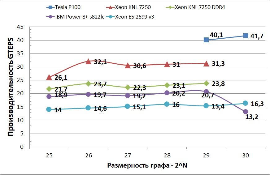
The graph below shows the average performance of the tested platforms. You can see that Power 8+ showed not very good stability when switching from a 64 GB to 128 GB graph. Perhaps this is due to the fact that used two socket node of two similar processors, and each processor had 128 GB of memory. And when processing a larger graph, part of the data was placed in a memory that did not belong to the socket. The graph also does not display the performance of the Tesla P100 on smaller graphs, since the difference between the fastest CPU device and the GPU is about 10 times. This acceleration is sharply reduced when the graphs become so large that they do not fit in the cache and the graph is accessed via NVlink. But, despite this limitation, the performance of the GPU still remains the most CPU of the devices. This behavior is explained by the fact that CUDA allows better control of computing and memory access, as well as better adaptability of graphics processors to parallel computing.

The table below illustrates the performance obtained in GTEPS / w on all test graphs. The table indicates the average power consumption with the average achieved performance on each of the graphs. The sharp drop in performance and energy efficiency during the transition from graph 2 ²⁸ to graph 2 ²⁹ on the NVidia Tesla P100 is due to the fact that there is not enough fast memory to place the aligned part of the graph that is most frequently accessed. If you use more memory (for example, 32 GB) and an increased communication channel with the NVlink 2.0 CPU, you can significantly improve the efficiency of processing large graphs.

Energy efficiency obtained in MTEPS / w:

Graph size	2 25	2 26	2 27	2 28	2 29	2 30
KNL 7250	121.4	149.3	142.33	136.56	130.96	N / A
E5 2699 v3	95.56	98.65	100	101.9	91.12	84.46
P8 + s822lc	93.8	97.04	93.2	95.28	92.41	53.23
Tesla P100	1228.57	1165.71	1235.96	1016.57	195.61	177.45

And finally

As a result of the work done, two parallel BFS algorithms were implemented for the CPU of similar systems and for the GPU. A study was conducted of the performance and energy efficiency of the implemented algorithms on various platforms, such as IBM Power8 +, Intel x86, Intel Xeon Phi (KNL) and NVidia Tesla P100. These platforms have different architectural features. Despite this, the first three of them are very similar in structure. Due to this, it is possible to run OpenMP applications on these platforms without any significant changes. On the contrary, the architecture of the GPU is very different from the CPU of similar platforms and uses a different concept for the implementation of computational code - the CUDA architecture.

Were considered graphs that are obtained after the generator for the Graph500 rating. The performance of each architecture on two data classes was investigated. The first class includes the graphs that are placed in the fastest memory of the calculator. The second class includes large graphs that cannot be placed in fast memory as a whole. To demonstrate energy efficiency, GreenGraph500 metrics were used. The minimal graph, which is taken into account in the GreenGraph500 rating in the big data class, contains 2 ³⁰ vertices and 2 ³⁴ edges and occupies 128 GB of memory in its original form. 2 ³⁰ 2 ³⁴ , , .

Graph500 GreenGraph500 NVidia Tesla P100 ( 220 GTEPS 1235.96 MTEPS/w), ( 41.7 GTEPS 177.45 MTEPS/w). NVLink, IBM Power8+.

NVidia Volta NVlink 2.0, .