Solution of the optimization problem of multistage rockets

Introduction

Nonlinear optimization methods are widely used in the design of machines and mechanisms. These methods are used in rocket production, for example, to optimize multi-stage rockets [1].

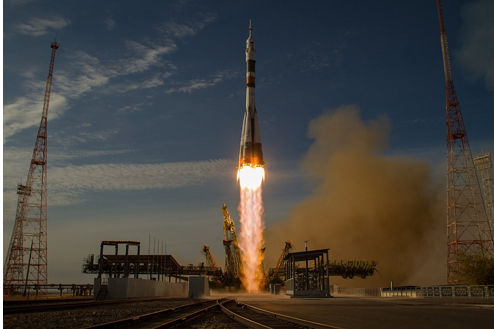
A multistage rocket is an apparatus in which parts of the structure are separated during flight, giving the remaining part of the rocket additional speed. A three-stage rocket is shown schematically in the figure.
')


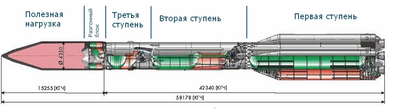
As the rocket moves, the stages separate until the main part of the rocket carrying the payload remains. The task of optimizing the rocket is to distribute the weight over the steps, at which a certain objective function reaches the maximum or minimum value.

We will consider two tasks on the assumption that the coefficient and the jet velocity Cn is constant at each stage, but at different levels it can take on different values. In both tasks, the payload ratio of the rocket G is taken as the target function, which must be minimized.

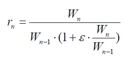
The characteristics of a multistage rocket can be described by two equations. The first equation for the payload ratio of a rocket:



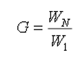
where: W1 is the useful weight of the rocket; WN is the initial weight of the rocket before the stages are separated.

The second equation for the characteristics of the payload of a multi-stage rocket, which can be written as an expression for its ideal final velocity (KE Tsiolkovsky formula):



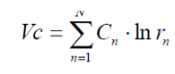
Where:



Consider a 4-stage rocket moving in the absence of a gravitational field with given values ​​of the ideal final velocity Vc , the initial weight of the rocket W4 , the jet velocity Cn and the coefficients Ɛn = Ɛ .

Setting goals

The first task is to find such a weight distribution in steps W3, W2 in order to minimize the payload ratio of the rocket G = W4 / W1 at a given speed Vc .

The second task is to find a weight distribution in steps W3, W2 in order to maximize the ideal final speed Vc for a given payload ratio of the rocket G.

Consider the first task of minimizing the payload ratio at a given rocket speed of Vc = 1,400 m / s and the speed of a jet stream Cn = C = 2000 m / s.

As control variables, we choose the weight distribution in steps: W3, W2 for given values ​​of the initial weight of the rocket W4 and the load effect coefficient n = = 0.3

Imagine a formula for calculating a given speed in the form:



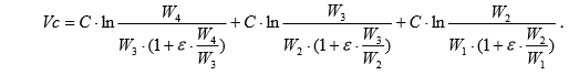
Where



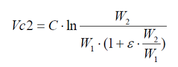
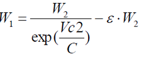
It follows that:



The solution to the first problem in Python

Python is a free high-level programming language. So far, optimization problems have been solved in the licensed math packages of Maple, Mathcad, Matlab and others.

Despite this, the arsenal of Python tools has wonderful numpy and scipy libraries. optimize, the use of which allows you to solve problems of conditional and unconditional, as well as custom optimization. However, their use requires careful selection of the initial conditions, the solver and the function of the goal, which we will now do.

I am listing the first part of the program, including the goal function:


Construct a contour graph of the goal function.


We get:



The complexity of the goal function consists in abrupt changes in the region of acceptable values ​​of variables, therefore we are exploring the from scipy library. optimize import minimize.

Usually, the goal function is written as [2]: fun = lambda x: (x [0] - 1) ** 2 + (x [1] - 2.5) ** 2 (example). Using such an entry in a solvable problem will complicate the analysis of the objective function. To simplify the notation of the target function, apply the auxiliary function fun2 (x):

 def fun2(x): return fun1(*x) 

We use the example from the documentation [2] for the SLSQP solver:

 import numpy as np from scipy.optimize import minimize import time start = time.time() def fun1(x,y): return 4000/(-0.3*y+y*np.e**(np.log(x/(0.3*x+y))+np.log(4000/(1200+x))-0.7)) def fun2(x): return fun1(*x) x0 =[3000,2000] #     res = minimize(fun2, x0, method='SLSQP', bounds=None) stop = time.time() print ("  :",round(stop-start,3)) print(res) 

We get the following result:

Optimization time: 0.0
fun: 8.8345830746128
jac: array ([7.71641731e-04, -4.12464142e-05])
message: 'Optimization terminated successfully.'
nfev: 48
nit: 12
njev: 12
status: 0
success: True
x: array ([2953.94929027, 1149.31138351])

We cannot vary the starting point of the search, for example, we have such a condition, therefore, to verify the optimality of the solution, we will rewrite the listing without specifying the method:

 import numpy as np from scipy.optimize import minimize import time start = time.time() def fun1(x,y): return 4000/(-0.3*y+y*np.e**(np.log(x/(0.3*x+y))+np.log(4000/(1200+x))-0.7)) def fun2(x): return fun1(*x) x0 =[3000,2000] #     res = minimize(fun2, x0)) stop = time.time() print ("  :",round(stop-start,3)) print(res) 

We get the following result:

Optimization time: 0.0
fun: 8.402280475718243
hess_inv: array ([[911166.17713172, 192191.3238931],
[192191.3238931, 194600.77394409]])
jac: array ([-1.19209290e-07, 1.31130219e-06])
message: 'Optimization terminated successfully.'
nfev: 152
nit: 28
njev: 38
status: 0
success: True
x: array ([1967.29278561, 967.91321904])

Time too, but the value of the goal function is less. Therefore, further searches can be stopped and present the final listing in the form:


We get the following result:

Optimizer operation time: 0.0
The estimated value of the objective function: 8.402
The change in weight of the rocket - 4000; 1967.293; 967.913; 476.061
Change the speed of the rocket -: 0; 466.785; 933.166; 1400.001



The weight of the rocket is distributed as follows (4000.0; 1967.0; 967.9; 476.1), which corresponds to an increase in speed in equal parts (after the separation of each step) by an average of 460 m / s.

We use the same formula for the final speed of the rocket, as in the previous problem:



Since W4 and W1 are set, the distribution of the weight of the rocket in steps W3 and W2 can maximize the ideal final speed Vc for a given payload ratio of the rocket G.

The solution of the second problem in Python

Taking into account the previously stated, we write down a part of the listing to the objective function:


Construct a contour graph of the goal function:


We obtain a contour graph of the target function with a negative sign to change the minimum to the maximum:



We got a local maximum (minimum on the chart), so the final listing will be presented in the form:


As a result, we get:

Optimizer running time: 0.016
The estimated value of the objective function: -1580.644
The change in the weight of the rocket -: 4000; 1473.625; 542.889; 200
Change the speed of the rocket -: 0; 526.873; 1053.753; 1580.64



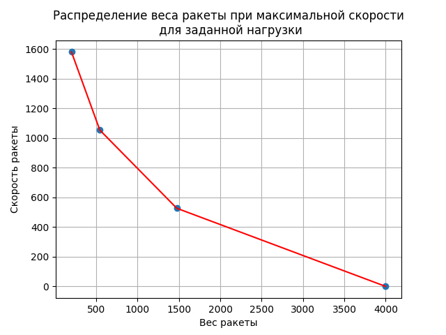
The rocket weights are distributed as follows: 4000; 1473.625; 542.889; 200, which corresponds to an increase in speed in equal parts (after separation of each stage) by 526.9 m / s.

findings

The publication describes the features of the use of the library scipy. optimize when solving optimization problems using the example of multistage rocket optimization. The results obtained in terms of the immutability of the initial point of the search for extremum for variables and the formation of a goal function in the usual user form will help expand the scope of the freely-available programming language Python.

Thank you all for your attention! And the main thing is that a multistage rocket with a load that is not useful for us NEVER arrives to us.

Links

1. Solving nonlinear programming problems
2. SciPy. Optimize.minimize