How to build an image classifier based on a pre-trained neural network
Now there is a process of democratization of artificial intelligence - technology, which has recently been considered the privilege of a limited number of large companies, is becoming increasingly available to individual professionals.
In recent years, a large number of models have appeared, created and trained by professionals using a large amount of data and huge computational power. Many of these models are in the public domain, and anyone can use them to solve their problems for free.
In this article we will analyze how the pre-trained neural networks can be used to solve the problem of image classification, and evaluate the advantages of their use.
')
Prediction of the class of plants on the photo
As an example, we will consider the problem of classifying images from the LifeCLEF2014 Plant Identification Task contest. The challenge is to predict the taxonomic class of a plant, based on several of its photographs.
We have 47815 images of plants available for training, each of which belongs to one of 500 classes. It is necessary to build a model that will return a list of the most likely plant classes. The position of the correct plant class in the list of predicted classes (rank) determines the quality of the system.
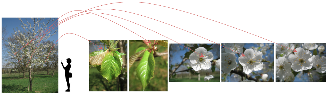
This task simulates a real life scenario where a person tries to identify a plant by studying its individual parts (stem, leaf, flower, etc.)
The model receives “observation” at the entrance - a set of photos of the same plant, made on the same day, using the same device, under the same weather conditions. As an example, you can take the image provided by the organizers of the competition:
Since the quality and quantity of photos varies from user to user, the organizers proposed a metric that will take into account the ability of the system to provide accurate predictions for individual users. Thus, a primary quality indicator is defined as the following average grade S:
Where - the number of users who have at least one photo in the test sample,
- the number of unique plants that the user has photographed ,
- A value from 0 to 1, calculated as the inverse of the rank of the correct class of the plant in the list of the most likely classes.
The competition banned the use of any external data sources, including pre-trained neural networks. We will intentionally ignore this restriction to demonstrate how the classifier can be improved with the help of pre-trained models.
Decision
To solve the problem, we will use neural networks that have been trained on 1.2 million images from the ImageNet database. The images contain objects belonging to 1000 different classes, such as a computer, a table, a cat, a dog, and other objects that we often meet in everyday life.
We chose VGG16, VGG19, ResNet50 and InceptionV3 as the base architectures. These networks were trained on a huge number of images and already know how to recognize the simplest objects, so we can hope that they will help us create a decent model for the classification of plants.
So let's start with ... image preprocessing, as without it.
Image preprocessing
Image preprocessing is pre-processing of images. The main purpose of preprocessing, in our case, is to identify the most important part of the image and remove unnecessary noise.
We will use the same preprocessing methods as the competition winners ( IBM Research team ), but with a few changes.
All images in the training set can be divided into categories depending on the part of the plant depicted in them: Entire (whole plant), Branch (branch), Flower (flower), Fruit (fruit), LeafScan (scan leaf), Leaf (leaf) , Stem (stem). For each of these categories was chosen its most suitable method of preprocessing.
Entire and Branch image processing
We will not change the Entire and Branch images, since often most of the images contain useful information that we don’t want to lose.
Example of whole images
 |  |
Sample Branch Images
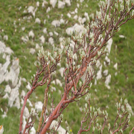 |  |
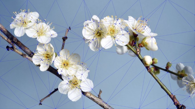
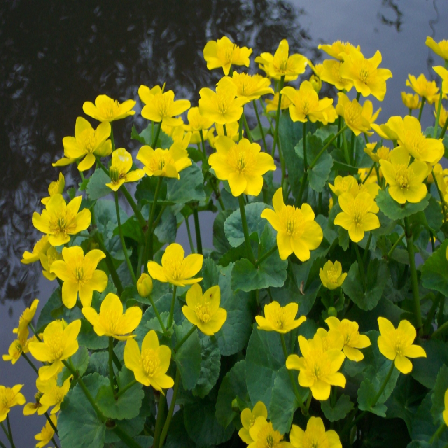
Processing Flower and Fruit images
We will use the same method for processing Flower and Fruit images:
- we convert the image to black and white;
- apply a Gaussian filter with the parameter a = 2.5;
- use the active contour method to find the most important part of the image;
- describe a rectangle around the border.
Example of processing a flower image
 |  |
Fruit image processing example
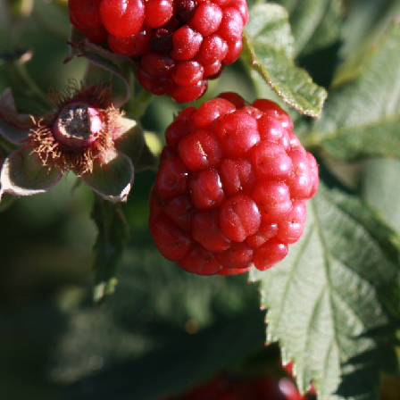 |  |
LeafScan Image Processing
Looking at LeafScan photos, you can see that in most cases the sheet is on a light background. We normalize the image with white:
- First, convert the image to black and white and use the Otsu-method to calculate the threshold value;
- all pixels whose values are less than the threshold value are painted white.
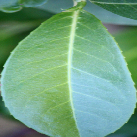
LeafScan Image Processing Example
 |  |
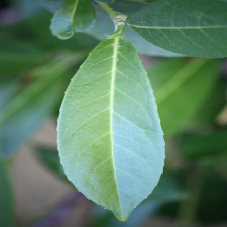
Leaf Image Processing
Usually in Leaf images, the sheet is in the center, and its outline is slightly receding from the edges of the image. For preprocessing such photos we will use the following method:
- cut out 1/10 of the image on the left, right, bottom and top;
- we convert the image to black and white;
- apply a Gaussian filter with the parameter a = 2;
- use the active contour method to calculate the boundary of the most important area;
- describe a rectangle around the resulting border.
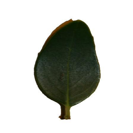
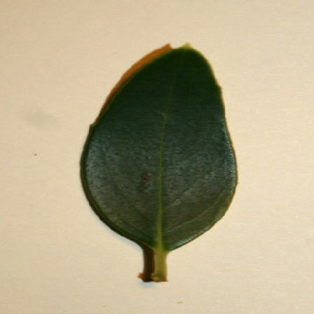
Leaf image processing example
 |  |
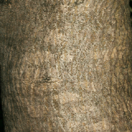
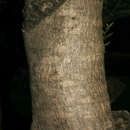
Stem image processing
The stem is usually located in the center of the image. To process Stem images we will use the following algorithm:
- delete ⅕ parts of the image on the left, right, bottom and top;
- we convert the image to black and white;
- apply a Gaussian filter with the parameter a = 2;
- use the active contour method to calculate the border of the most important image area;
- describe a rectangle around the resulting border.
Stem image processing example
 |  |
Now everything is ready for building a classifier.
How we built an image classifier based on a pre-trained neural network
We will build the model using Keras with TensorFlow as a back-end. Keras is a powerful machine learning library designed to work with neural networks, which allows you to build all kinds of models: from simple ones, such as a perceptron, to very complex networks designed for video processing. And what is very important in our case, Keras allows you to use pre-trained neural networks and optimize models using both the CPU and the GPU.
STEP 1
First, we load the pre-trained model without fully connected layers and apply the pooling operation to its output. In our case, the best results were shown by the “average” pooling ( GlobalAveragePooling ), and we will take it for building a model.
Then we run the images from the training set through the resulting network, and save the received signs to a file. A little later, you will see why it is needed.
STEP 2
We could freeze all layers of the pre-trained network, add our fully connected network over it, and then train the resulting model, but we will not do that, because in this case we will have to drive all the images through the pre-trained network at each epoch, a lot of time. To save time, we use the features that we saved in the previous step in order to train a fully connected network on them.
At this stage, do not forget to divide the training set into two parts: the training set in which we will be trained, and the validation set in which we will consider an error in order to correct the weights. Data can be divided in the ratio of 3 to 1.
Let's take a closer look at the full mesh network architecture that we will be teaching. After a series of experiments, it was found that one of the best architectures has the following structure:
- 3 dense layers of 512 neurons. Behind each dense layer is a dropout layer, with a parameter of 0.5. This means that in each layer on each pass of the network, we randomly emit signals of about half of the neurons;
- the output layer is softmax for 500 classes;
- as a loss function, we use categorical cross-entropy , and we optimize the network with Adam ;
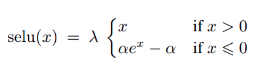
- It was also noted that using the selu function (scaled exponential unit) instead of relu as an activation function helps the network converge faster.
Useful information:
- with the described learning method, we cannot use augmentation (image transformation: rotations, compression, adding noise, etc.), but since the model obtained at this step is only an intermediate result in the process of creating the final model, for us this limitation is not critical;
- such networks learn very quickly, and we can manually determine the required number of epochs;
- in our case, the neural network required 40 to 80 epochs for convergence;
retraining or under-training of a model should not worry us much, since we will still have a chance to fix it.
STEP 3
In this step, we add a trained fully meshed network on top of the pre-trained model. The loss function is left unchanged, and we will use another optimizer for network training.
The pre-trained neural network has already learned a lot of abstract and common features, and in order not to knock down the found weights, we will train the network with a very small learning rate. Optimizers such as Adam and RMSProp themselves select the learning speed, in our case, the selected speed may be too high, so they do not suit us. To be able to set the learning speed by ourselves, we will use the classic SGD optimizer.
To improve the quality of the final classifier, you need to remember the following:
- reduce the learning rate on the plateau so as not to go too far towards the minimum ( ReduceLROnPlateau callback );
- if over several epochs the error on validation data does not decrease, then it is worth stopping training ( EarlyStopping callback );
- Usually, additional training of models takes a lot of time and when we close .ipynb files, all dynamic output is lost. I recommend saving the training information to a file ( CSVLogger callback ) so that you can further analyze how the model is being trained.
Instead of the standard progress bar, I prefer to use TQDMNotebookCallback . This does not directly affect the result, but it’s much more pleasant to watch model training with it.
Data augmentation
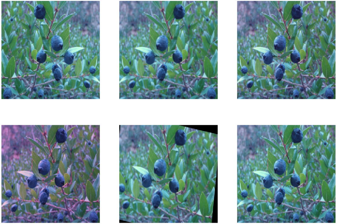
Because in the final step we train the entire network, here we can use augmentation. But instead of the standard ImageDataGenerator from Keras, we will use Imgaug - a library that is designed to augment images. An important feature of Imgaug is that you can explicitly indicate with what probability the transformation should be applied to the image. In addition, in this library there is a wide variety of transformations, it is possible to combine transformations into groups, and choose which of the groups to apply. Examples can be found at the link above.
For augmentation, we select those transformations that can occur in real life, for example, mirroring photos (horizontally), turns, zoom, noise, change in brightness and contrast. If you want to use a large number of transformations, it is very important not to apply them at the same time, since it will be very difficult for the network to extract useful information from the photo.
I propose to split the transformations into several groups and apply each of them with a given probability (each may have a different probability). I also recommend augmenting images in 80% of cases, then the network will be able to see the real images. Given that training takes several dozen epochs, there is a very big chance that the network will see each image in the original.
Accounting for user ratings of photos
The metadata for each image contains a quality rating (average user rating, showing how well the image is suitable for classification). We assumed that images with a score of 1 and 2 are quite noisy, and although they may contain useful information, in the end, they may adversely affect the quality of the classifier. We tested this hypothesis while training InceptionV3. There were very few images with a rating of 1 in the training set, only 1966, so we decided not to use them in training. As a result, the network has been trained better in images with a rating higher than one, so I recommend that you carefully consider the quality of the images in the training set.
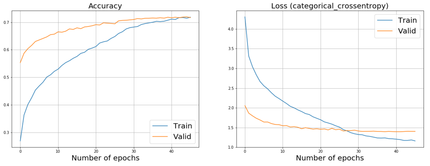
Below you can see the graphs of additional training ResNet50 and InceptionV3. Looking ahead a bit, I’ll say that it was these networks that helped us achieve the best results.
ResNet50 Advanced Training Schedule
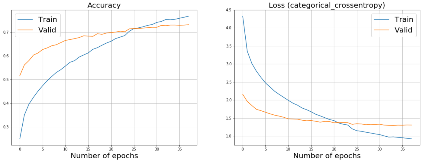
InceptionV3 Advanced Training Schedule
Test time augmentation
Another way to help increase the quality of the classifier is prediction on augmented data (test-time augmentation, TTA). This method consists in making predictions not only for images in the test set, but also for their augmentations.
For example, take the five most realistic transformations, apply them to the images and get the predictions not for just one picture, but for six. After that, we average the result. Please note that all augmented images are obtained as a result of one transformation (one image - one transformation).
An example of prediction augmentation
results
The results of the work done are presented in the table below.
We will use 4 metrics: the main metric proposed by the organizers, as well as 3 top metrics - Top 1, Top 3, Top 5. Top metrics, like the main one, are applied to the observation (a set of photos with the same Observation Id), and not to a separate image.
In the process, we tried to combine the results of several models in order to further improve the quality of the classifier (all models were taken with the same weight). The last three lines in the table show the best results obtained when combining models.
| Model | Network | Target metric (rank) | Top 1 | Top 3 | Top 5 | Epochs | Tta |
|---|---|---|---|---|---|---|---|
| one | VGG16 | 0.549490 | 0.454194 | 0.610442 | 0.665546 | 49 | Not |
| 2 | VGG16 | 0.553820 | 0.458732 | 0.612600 | 0.666996 | 49 | Yes |
| 3 | VGG19 | 0.559978 | 0.468980 | 0.620219 | 0.671253 | 62 | Not |
| four | VGG19 | 0.563019 | 0.470534 | 0.619303 | 0.676396 | 62 | Yes |
| five | ResNet50 | 0.573424 | 0.489943 | 0.627836 | 0.682585 | 46 | Not |
| 6 | ResNet50 | 0.581954 | 0.495962 | 0.638806 | 0.688938 | 46 | Yes |
| 7 | InceptionV3 | 0.528063 | 0.495962 | 0.666928 | 0.716630 | 38 | Not |
| eight | InceptionV3 | 0.615734 | 0.535675 | 0.671392 | 0.723992 | 38 | Yes |
| 9 | Combining models 1, 3, 5, 7 | 0.63009 | 0.549993 | 0.677204 | 0.721084 | - | - |
| ten | Combining models 2, 4, 6, 8 | 0.635100 | 0.553577 | 0.680857 | 0.727824 | - | - |
| eleven | Combining models 2, 6, 8 | 0.632564 | 0.551064 | 0.684839 | 0.730051 | - | - |
The competition winners model showed a score of 0.471 in the target metric. It is a combination of statistical methods and a neural network, trained only on those images of plants that were provided by the organizers.
Our model, which uses the pre-trained neural network InceptionV3 as the basis, achieves the result of 0.60785 in the target metric, improving the result of the contest winners by 29%.
When using augmentation on test data, the result on the target metric increases to 0.615734, but at the same time, the model's speed drops by about 6 times.
We can go even further and combine the results of several networks. This approach allows to achieve the result of 0.635100 on the target metric, but at the same time the speed drops very much, and in real life such a model can be used only where work speed is not a key factor, for example, in various studies in laboratories.
Existing models can not always correctly determine the class of the plant, in this case it may be useful to know the list of the most likely plant species. In order to measure the ability of a model to produce the true class of a plant in the list of the most likely classes, we use top metrics. For example, according to the Top 5 metric, the InceptionV3 learned network showed a result of 0.716630. If we combine several models and apply TTA, then we can improve the result to 0.730051.
I described how we managed to improve the quality of the model using pre-trained neural networks, but, of course, this article describes only a part of the available methods.
I recommend trying other approaches that look quite promising:
- the use of more accurate methods for image processing;
- modification of the architecture of fully connected layers;
- change of activation function for dense layers;
- using only the highest quality images for training (for example, with a rating higher than 2);
- the study of the distribution of classes in the training set, and the use of the class_weight parameter during training.
Total
Additional training of neural networks, which were trained on more than 1 million images, has significantly improved the solution presented by the winners of the competition. Our approach has shown that pre-trained models can significantly improve the quality of image classification problems, especially in situations where there is not enough data to train. Even if your basic model has nothing to do with the problem to be solved, it may still be useful, since it already knows how to recognize the simplest objects of the surrounding world.
The most important steps that helped achieve these results:
- using Imgaug for image augmentation (this library contains more transformations than the Keras ImageDataGenerator , in addition, it is possible to combine transformations into groups);
- 80% of images were augmented at each training epoch;
- the use of predictions on augmented data (TTA);
- decrease in learning rate on the plateau;
- stop learning if the value of the loss function on validation data does not decrease over several epochs;
- model training on images with a score greater than 1.
I wish you good luck in your experiments!
Source: https://habr.com/ru/post/344222/
All Articles