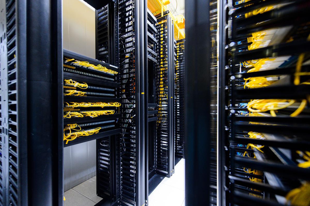
Monitoring of engineering infrastructure in the data center. Part 4. Network infrastructure: physical equipment
Part 1. Monitoring of engineering infrastructure in the data center. Highlights.
Part 2. How is the monitoring of power supply in the data center.
Part 3. Monitoring of cold supply by the example of the NORD-4 data center.
Part 4. Network infrastructure: physical equipment.
Hi, Habr! My name is Alexey Bagaev, I am the head of the network department in the DataLine.
')
Today, I will continue a series of articles on monitoring the infrastructure of our data centers and talk about how we have organized network monitoring. This is a fairly voluminous topic, so in order to avoid confusion, I have divided it into two articles. This discussion will focus on monitoring at the physical level, and next time we will look at the logical level.
First, I will describe our approach to network monitoring, and then I will tell you in detail about all the parameters of network equipment that we monitor.
Content:
Our approach
Network monitoring and network monitoring
Network Hosts Status
Temperature readings
Status of the fans in the switches
Power Module Status
Port status
Processor status
Control Plane Policy: the effect of traffic on CPU usage
RAM monitoring
Small bonus
Our approach
Our practice of “monitoring everything” has been going on for more than five years. In some areas we do not reinvent the wheel and act by standard methods, but somewhere, by virtue of specificity, we resort to our solutions. In particular, this concerns the monitoring of the logical level of the network, but, as I said earlier, this is the topic of a future article.
In the case of polling the physical layer of the network, everything is quite simple. The monitoring system of the network infrastructure is based on the open-source tools of Nagios and Cacti. Just in case, let me remind them of their differences: Nagios records events in real time, and Cacti aggregates statistics, builds graphs and tracks the dynamics of indicators in the long term.
The state of the network equipment is monitored through requests using the standard SNMP protocol:
request server – agent: GetRequest and agent – server: Trap.
In the OS of all managed network equipment there are MIB-bases. The required OID of the object, as a rule, we find using the SNMPWalk command or using the MIB Browser tool. You can follow this link to the English branch Reddit, in the comments there are several sensible recommendations on this topic.
Of course, the equipment is periodically changing and modernizing, and we are updating the monitoring system for new tasks. Before entering a new host into the product, in parallel with testing, we add this host to the monitoring system and determine the list of objects that we will be tracking.
We collect the main metrics of the connected equipment, from the most elementary it is a check for UP / DOWN .
In general, we are interested in:
- external factors (temperature, nutrition, etc.);
- port status (current state, availability);
- processor status;
- memory;
- specificity of "iron" depending on the type of equipment.
It cannot be said that a node is more important than the others. The productive network is also productive in Africa. “Clogged” memory or an overloaded processor can cause network degradation in general and customer problems in particular. Macro task in monitoring network iron - timely prevention and troubleshooting before they make themselves known.
Network monitoring and network monitoring
In monitoring the network, we use two ways to access equipment: in-band and out-of-band . Out-of-band is preferable for us: with such a scheme, the traffic of the monitoring system does not follow the productive links that are used to provide services to customers.
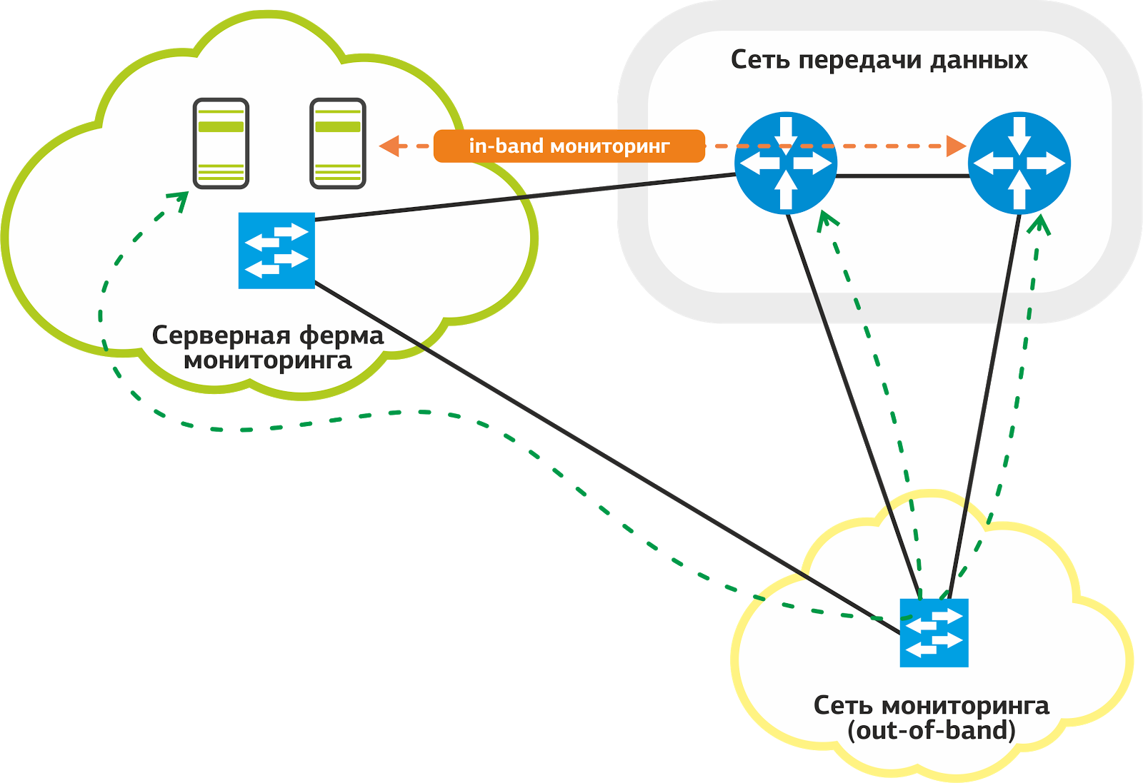
Our monitoring network.
We have a special network for monitoring: it is connected by dedicated links to the ports on each network host. Even if there are problems with productive links, monitoring will work without fail.
It often happens that the problem on one link makes a significant part of the network inaccessible for monitoring. This complicates the work of the support service and slows down the troubleshooting process. The out-of-band scheme solves this problem.
Not all hosts manage to connect out-of-band , and in these cases we use in-band when monitoring traffic goes along with productive. Oddly enough, despite the obvious shortcomings of this scheme, it has its advantage - reliability.
Productive links are backed up by protocols at the L2 and L3 level: if the main link fails, traffic “moves” to another link. Nagios can react to this with a flap of services, but the support service will remain in monitoring.
Then I will go in order for all the monitoring nodes of the physical network equipment.
Network Hosts Status
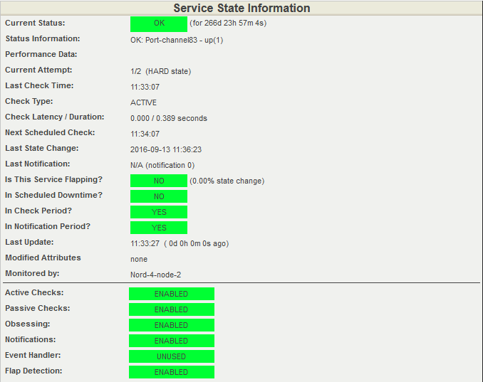
We check the availability of the host by sending ICMP requests to its management IP addresses. Typically, this is a dedicated IP in the equipment control network.
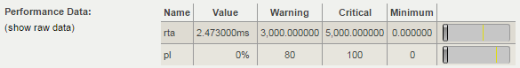
Once a minute, the host is checked by running the check_ping plugin for Nagios. Each call is followed by sending four ICMP requests at 1 second intervals. The screenshot below shows that the last check was completed with a result of 0% packet loss. The average response time of the RTA (round trip average) was 2.47 milliseconds. This is the norm.
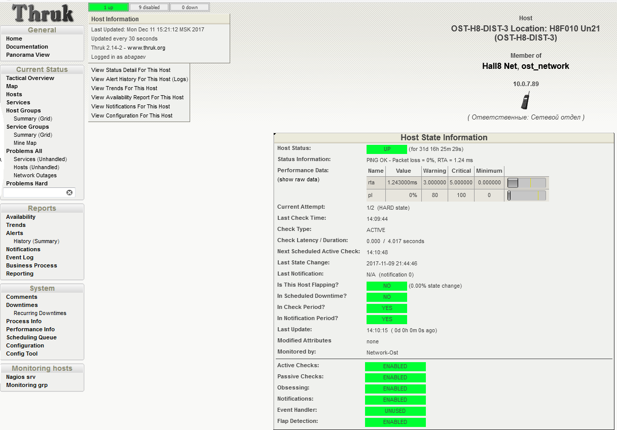
Check the status of the host. UP status: 0% packet loss, average RTA time 2.47 ms. UPD:
screenshot changed, thanks for editing Tortortor
How do we understand that a malfunction has occurred? Of course, it is impossible to entrust the monitoring of all the numbers to the common man: engineers monitor the condition of the equipment in the convenient interface of Nagios. It has already set proven thresholds for triggering the status of WARNING (approaching undesirable indicators) and CRITICAL (critical threshold exceeding, expert intervention is required).
Take a close look at the Performance Data table from the previous screenshot: the Value column contains the current value of the Packet loss parameter. WARNING is issued when reaching 80% of the lost packets of the total number of sent, CRITICAL - at 100. The RTA (Round Trip Average), equal to 2.47 ms, means the average response time. A warning will be issued upon reaching 3 ms, the critical threshold is set to 5 ms.
On the same screen, you can get a brief summary of the following indicators:
- Next Scheduled Active Check - the time of the next check;
- Last State Change - when the state was last changed;
- Last Notification - the last notification issued by the system;
- Is Scheduled Downtime - Whether the inactivity time is scheduled.
Temperature readings
Recently, my colleagues talked about the monitoring of cold supply in machine rooms, where they mentioned that for each cold corridor there are three temperature sensors. These sensors take the overall performance along the corridor and make it possible to judge the operation of the cooling system itself.
To monitor the network infrastructure, you need to know the readings of the temperature sensors from each piece of equipment. This allows you to identify and eliminate not only possible overheating of the hosts, but also to determine at the early stage local overheating of the racks.
To get the status of the device, we send a request of the form snmpwalk <parameters> <device> | grep <what are we looking for> and get a list of all OIDs by the specified filters.
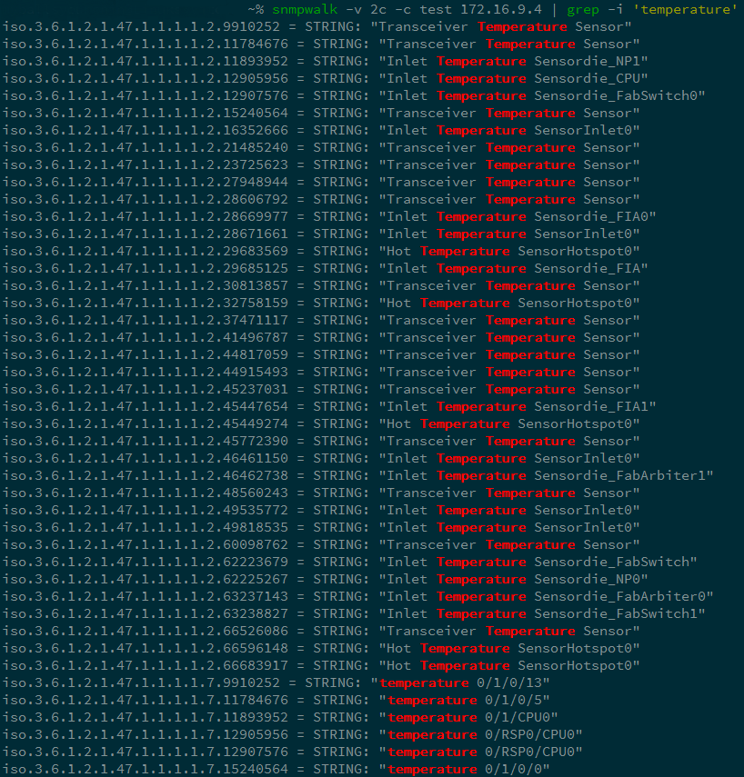
Request temperature readings on the Cisco ASR9006 router.
Having studied the conclusion, we make a more detailed request:
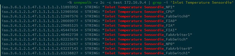
Make a request parameter Inlet Temperature Sensordie to remove the temperature values.
And even more detailed:
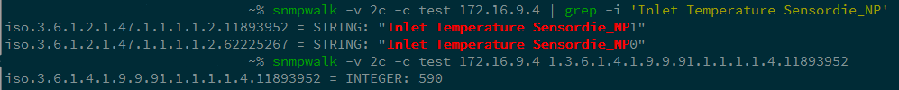
Select the parameters NP1 and NP2.
As a result, we get the OID 1.3.6.1.4.1.9.9.91.1.1.1.1.4.index and we can track the readings of the desired temperature sensor. In our example, the value is 590, i.e. 59 degrees Celsius.
In the graphical representation of Nagios, the survey results are as follows:
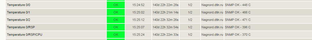
In the screenshot we see the following:
- Temperature 0/0, 0/1, 0/2 - line card sensors of the ASR9006 router;
- RSP - sensor card Route Switch Processor;
- RSP / CPU - CPU temperature sensor of the Route Switch Processor card.
Status of the fans in the switches
To ensure that the equipment does not overheat, we use the cooling system of our data center and the system of cold and hot corridors to ensure a constant flow of air into the rack from the cold corridor and simultaneous “blowing out” of the heated air into the hot corridor. The role of “pumps” that pump air through the equipment is performed by the fans inside the switches — not to be confused with the fans on the racks. We monitor their status to prevent equipment overheating.
If the fan stops, we will have a certain amount of time to replace it, otherwise the equipment may suffer.
To get the current status of the fan, make a request similar to the one above:
iso.3.6.1.4.1.9.9.117.1.1.2.1.2.24330783 = INTEGER: 2
Answer 2 means ON. The fan works, Nagios does not panic.
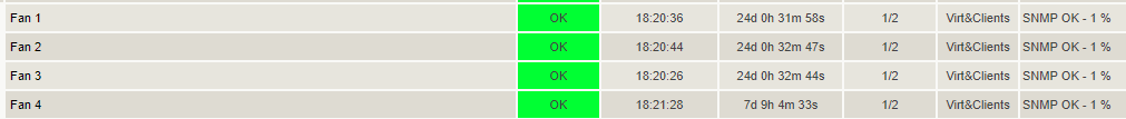
This displays the status of the fans in Nagios.
A small remark: when setting up monitoring systems, our specialists use the values obtained under test loads and “crash tests” as threshold values. Getting out of the "normal" range warns of an impending problem, and we have time to "smooth" troubleshooting. At the same time, in many cases, in real time, we have a rather simple indication of “working / not working”.
Power Module Status
This indicator is very obvious and does not need comments. We only mention that the alert system will inform us about the malfunction and / or lack of power in the power supply units of the network equipment themselves.
If the power is lost, the service on duty will quickly figure out the reason. This could be a problem with the power cable, a lack of power at this input, or a problem directly with the unit itself. Having received the notification, the engineer will take measures and restore the normal operation of the equipment.
Power Modules OID: 1.3.6.1.4.1.9.9.117.1.1.2.1.2.index
We send a request and get the status: iso.3.6.1.4.1.9.9.117.1.1.2.1.2.53196292 = INTEGER: 2
Power module is OK.
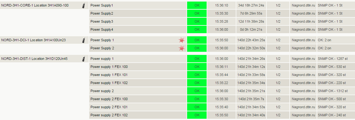
So the state of the power modules is monitored at Nagios.
Port status
To track backbone and subscriber connections, we monitor the following parameters:
- port availability;
- signal level (for optical ports);
- traffic volume (port speed);
- mistakes.
I'll tell you about each parameter separately.
To check the operational status of the port, we produce a standard OID request.
Enter the OID of the desired port: 1.3.6.1.2.1.2.2.1.8.ififdex
We get the answer: iso.3.6.1.2.1.2.2.1.8.1073741829 = INTEGER: 2
Visualization of the answer in Nagios.
If the port is optical, check the signal level on the optics.
1. Check the outgoing signal:
OID: 1.3.6.1.4.1.9.9.91.1.1.1.1.4.txindex
Answer: iso.3.6.1.4.1.9.9.91.1.1.1.1.4.6869781 = INTEGER: 8580
2. Then we check the incoming signal:
OID: 1.3.6.1.4.1.9.9.91.1.1.1.1.4.rxindex
Answer: iso.3.6.1.4.1.9.9.9.11.1.1.1.4.63630989 = INTEGER: 2499
Decipher the numbers in the examples above. The request returns the value in milliwatts to us and shows four decimal places. That is, the figures above mean 0.8 mW and 0.2 mW. Next, the built-in function of the Cacti template converts the value to dBm (decibel-milliWatt).
Statistics on attenuation levels on optical links is useful when analyzing network problems. Cacti allows you to see the dynamics of degradation and find the cause of problems on the link.
We had an unusual case with a signal on one of the optical paths. The graph below shows a dip in the optical signal reception level. This failure lasted a whole week, but then the level abruptly “bounced off” to its normal state. What could it be, we can only guess. Perhaps some contractor did work in the telephone sewer, and then quietly returned everything to the site.
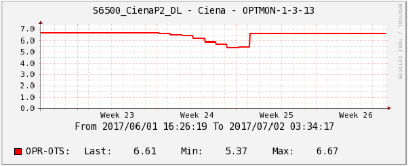
Signal statistics on the optical path in Cacti.
Another very important parameter is the throughput (speed) of the ports. We need to get real-time information about the degree of congestion of network links.
This metric allows us to plan traffic and manage network capacity. In addition, with statistics on link throughput, we can analyze the effects of a DDoS attack and take steps to reduce the impact of DDoS attacks in the future.
To get a summary of the number of received and sent packets of information, we use the queries again:
1. Received packages
OID: 1.3.6.1.2.1.31.1.1.1.6.ifindex
Answer: iso.3.6.1.2.1.31.1.1.1.6.1073741831 = Counter64: 109048713968
2. Sent packages
OID: 1.3.6.1.2.1.31.1.1.1.10.ifindex
Answer: iso.3.6.1.2.1.31.1.1.1.10.1073741831 = Counter64: 67229991783
The numbers received in the queries above are the number of bytes. The difference in these values for N seconds / N is the bandwidth in bytes. If we multiply by eight, we get the bit / s. Those. monitoring requests a value once a minute, compares it with the previous one, calculates the difference between two values, translates a byte into a bit and obtains the bit rate / s.
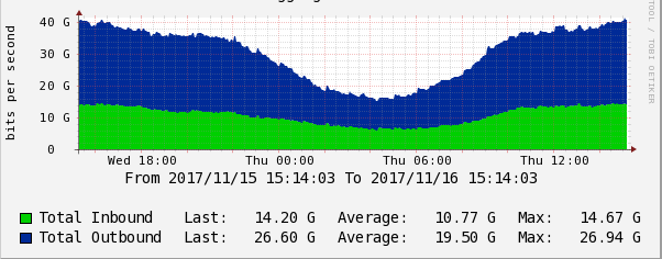
Graph of data transfer rate in Cacti.
Often, our subscribers experience the degradation of Internet channels due to the overflow of the bandwidth allocated for them. It is difficult to immediately determine the cause of degradation: a symptom on the subscriber’s side is partial packet loss. To quickly recognize this problem in Nagios, we set the trigger thresholds to the bandwidth of each subscriber channel.
In the Nagios dashboard it looks like this:

Detailed output:
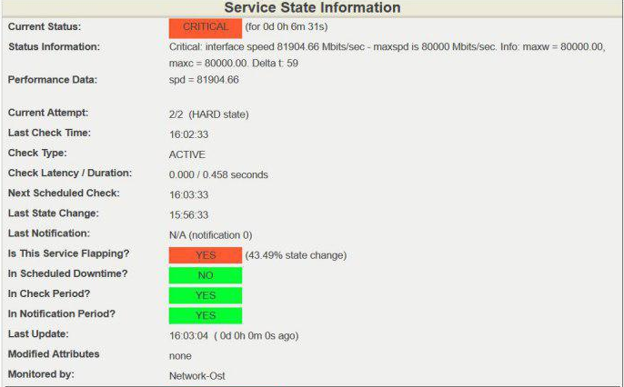
Exceeding the 80 Gbit / s speed threshold on a 100-gigabit channel is considered dangerous; in such cases, we take measures to unload the channel or expand it. Remember, you always need to leave “space for maneuver”, i.e. free bandwidth in case of rapid traffic growth. This may be the peak attendance of a resource, backup or, in the worst case, DDoS.
Finally, we monitor errors for each port. Using error statistics, we localize and fix the problem.
1. Find out the number of received packets with errors:
OID: 1.3.6.1.2.1.2.2.1.14 . Ifindex
Answer: iso.3.6.1.2.1.2.2.1.14.1073741831 = Counter32: 0
2. Check the number of packages that were not sent, because contained errors:
OID: 1.3.6.1.2.1.2.2.1.20.ifindex
Answer: iso.3.6.1.2.1.2.2.1.20.1073741831 = Counter32: 0
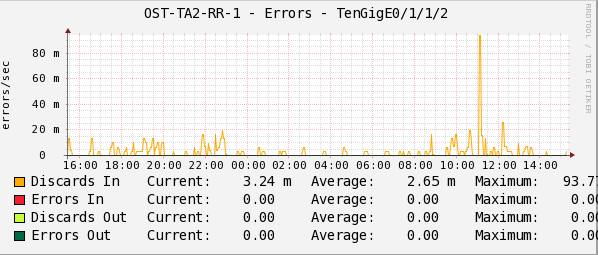
Statistics in Cacti records the number of errors in the transmission of packets per second.
The indicators Discards In / Out and Errors In / Out on the chart are consolidated counters of all the possible reasons why the data packet could not be transmitted to higher-level protocols.
To track errors and find out about problems with links, Nagios has an alert system for each OID. However, errors can not always be traced promptly, therefore, in order to timely notify the engineers on duty, Nagios has additionally configured a service for monitoring errors at ports.
This is how error checking on ports in Nagios looks like.
Perhaps these are all the key metrics of the ports that we monitor.
I will mention only one important point: when you restart a switch with a Cisco IOS operating system, for example Cisco Catalyst 6500, the port-ifindex correspondence changes. This inevitably leads to the need to reconfigure SNMP requests in the monitoring system. To fix the interface index values (ifindex), you need to enter the snmp ifmib ifindex persist command in global IOS mode, then after reloading the ifindex in the MIB will remain unchanged.
Processor status
A processor load close to 100% can adversely affect the health of a network host or the network as a whole. This is the case when we should instantly find out about exceeding the allowable thresholds. For this, as you already understood, we use Nagios. Studying the graphics from Cacti and watching the system in real time, we understand the trends and cyclical operation of the processors. All this helps engineers to find and neutralize problems before they affect the network.
We make a request for the state of the processor of network devices:
OID: 1.3.6.1.4.1.9.9.109.1.1.1.1.7.index
Answer: iso.3.6.1.4.1.9.9.109.1.1.1.1.7.2098 = gauge32: 2
We get the CPU load per minute.

CPU load status in Nagios.
Open detailed information about the state of the processor. Again, look at the Performance Data item in the screenshot below. It contains information on the current processor load and threshold values. The current load is 3%. The warning system will give a 50% load and will give a CRITICAL signal at 70% load.
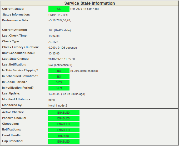
Detailed information about the state of the processor. All indicators are normal.
Control Plane Policy: the effect of traffic on CPU usage
This indicator complements the above basic information on CPU usage. Part of the incoming traffic is processed by the processor, and we track its type and quantity separately. An increased CPU load can be caused by a DDoS attack, as well as quite valid traffic (ICMP, ARP requests, etc.), which is simply too much.
Processing an excessive amount of data, any processor can boot "to the eyeballs" and can not handle service traffic, such as routing protocols - routing updates or hello / keepalive-packages . Accordingly, the interaction with the neighboring network equipment will stop, and the service will degrade or fall.
Here is a real example:
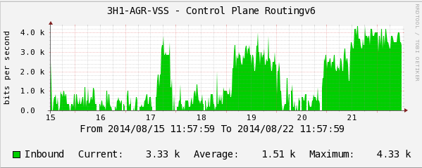
IPv6 routing protocol packet rate.

CPU Load Schedule.
The graphs show how IPv6 routing protocol packets begin to load the switch CPUs. This fact can be overlooked in a timely manner and with an increase in the flow of IPv6-packets to get a very painful incident on the network.
Using stress tests on network equipment, we determined which traffic by type and number leads to problems on network devices, and we set the optimal threshold values for each of them to control plane policing . The graphs below show jumps in the values above the threshold.
An example of monitoring CoPP (control plane policing) on one of the switches in production:
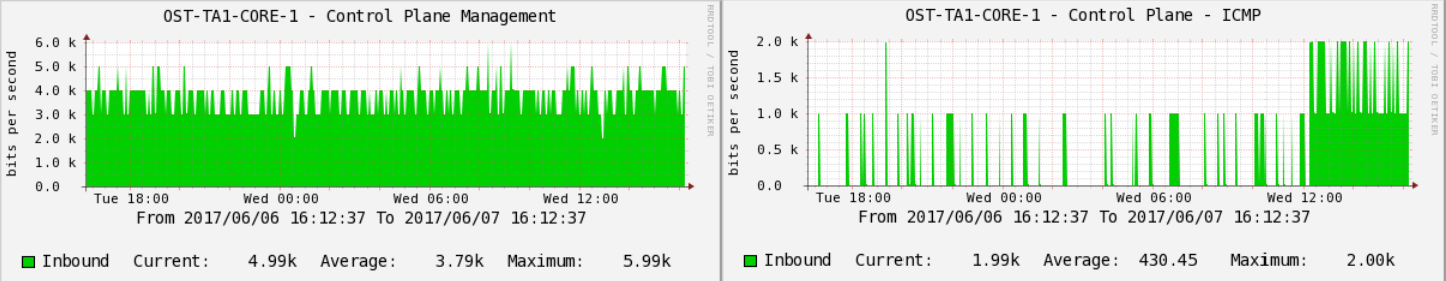
The number of bits per second of traffic packets. ICMP going to CPU processing.
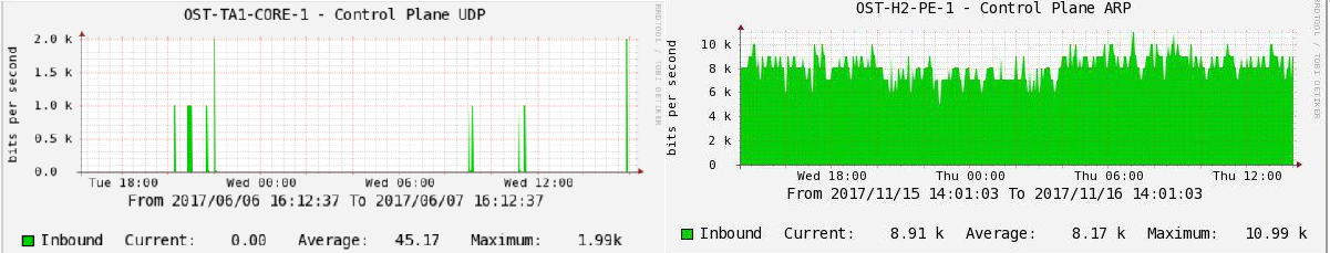
UDP packets.
Observing these indicators, we can prevent the increased load on the processor and maintain the stability of the network. As is the case with the rest of the monitoring data, we collect history using Cacti and display the current situation on monitors using Nagios.
RAM monitoring
One of the most dangerous situations in the case of RAM is memory leak. It is important to warn and eliminate it in a timely manner, as in small intervals (day, week) a slow but inevitable decrease in free memory can simply be overlooked.
Partially solve this problem allows the collection of long-term statistics in Cacti. We can track down memory overflows and plan a technology window for rebooting equipment. Unfortunately, in most cases, this is the only absolute method to “cure” a leak.
Here is another example from the life of our network:
During the next analysis of monitoring indicators, engineers discovered the dynamics of decreasing the amount of free memory on one of the switches. The changes were almost imperceptible at short intervals of time, but if we increase the time scale, say up to a month, there appeared a trend towards a gradual decrease in free memory. When memory is full, the consequences for the switch can be unpredictable, even to the oddities in the behavior of routing protocols. For example, part of the routes may cease to be announced to its neighbor. Or it will randomly start to refuse peer-link on the VSS system.
The situation described above ended quite well. We agreed with the customers of the technical window and overloaded the switch.
So let's continue. Cacti plots help determine the exact time of the start of a leak, and by comparing the logs, we find and “cure” the cause.
Make a request to load RAM:
OID: 1.3.6.1.4.1.9.9.221.1.1.1.1.18.index
The answer: iso.3.6.1.4.1.9.9.221.1.1.1.1.18.52690955.1 = Counter64: 2734644292
The value indicates the number of bytes from the memory pool used by the operating system.
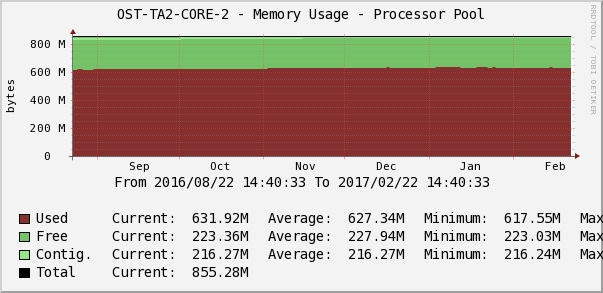
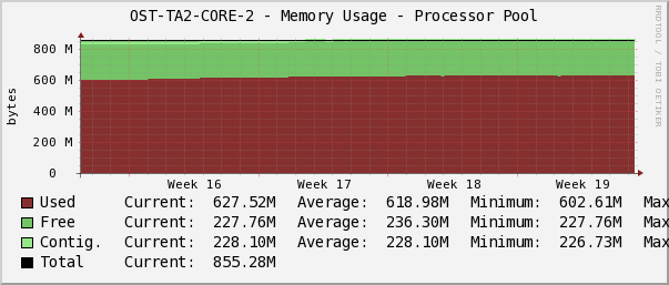
Statistics of loading RAM in Cacti.
The engineer on duty ensures that there are no anomalous drops or a trend for permanent filling of free memory using the Memory Usage parameter. The graph in Cacti shows memory for processes, I / O, shared memory, the amount of free / used memory.
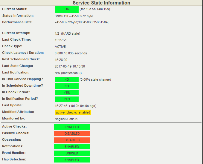
The current value of the free RAM of the switch is unloading from Nagios.
At the time of the creation of the screenshot, 45503272 bytes of the OP were free, the response thresholds were set: for WARNING - in the range from 35651584 to 39845888 bytes, for CRITICAL - from 0 to 35651584 bytes.
Small bonus
I will write a few words about how the monitoring system alerts us to emergency situations.
In our own "kitchen" we do not use additional email or SMS alerts, as the engineers on duty do an excellent job with monitoring the indicators on the screens. The exceptions are some critical indicators, about the changes that we need to know immediately and regardless of the human factor. For these indicators, we set up an e-mail or SMS distribution. At the request of the client, we can set up separate alerts for each response. Here everything is individual. When any parameter in Nagios reaches the hard state, the system notifies the customer through the channel that we set up for it.
And one more trifle, but pleasant. The monitoring system not only allows you to quickly respond to events, but also helps the attendants to quickly resolve the problem. We do this by placing a link to the instructions on the host or the Nagios service:

The link to the resource with the instruction is under the icon “Red Book” (View Extra Host Notes), as a knowledge base with instructions we use Redmine. The duty officer can follow the link and clarify the sequence of actions for troubleshooting. On the left in the screenshot there is a picture in the form of a phone, it is possible to find out the department responsible for this service, and, in case of difficulties, the incident escalates to this division of the production directorate.
In conclusion, I want to draw your attention to the rather critical vulnerability of the SNMP protocol (versions 1, 2c and 3) in the Cisco IOS and XE operating systems. The vulnerability allows an attacker to gain complete control over the system or initiate a reboot of the operating system of the attacked host. Cisco announced the vulnerability on June 29, 2017, and it was closed in new software releases released after mid-July. If it is not possible to update the software for any reason, as a temporary solution, Cisco recommends that you disable the following MIB bases:
- ADSL-LINE-MIB
- ALPS-MIB
- CISCO-ADSL-DMT-LINE-MIB
- CISCO-BSTUN-MIB
- CISCO-MAC-AUTH-BYPASS-MIB
- CISCO-SLB-EXT-MIB
- CISCO-VOICE-DNIS-MIB
- CISCO-VOICE-NUMBER-EXPANSION-MIB
- TN3270E-RT-MIB
This monitoring network infrastructure hardware ends. Ask questions in the comments, and I’ll tell you about monitoring the network infrastructure at the logical level next time.
Source: https://habr.com/ru/post/344188/
All Articles