Convolution network in python. Part 2. Derivation of formulas for training models

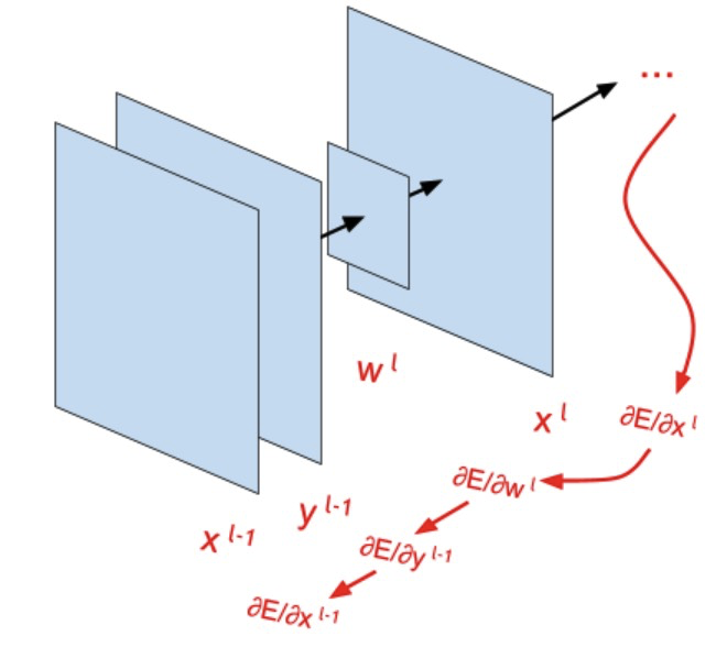
In the last article, we examined conceptually all the layers and functions of which the future model will consist. Today we will derive formulas that will be responsible for teaching this model. Layers will be disassembled in reverse order - starting with the loss function and ending with the convolutional layer. If there are difficulties in understanding the formulas, I recommend that you familiarize yourself with the detailed explanation (in the pictures) of the error back-propagation method, and also recall the rule of differentiation of a complex function .

Derivation of a formula for back propagation of an error through the loss function

This is just a partial derivative of the loss function.

E

$E$ on the exit model.

\ begin {array} {rcl} \ dfrac {\ partial E} {\ partial y ^ {l} _ {i}} & = & \ dfrac {\ partial \ frac {1} {2} \ sum_ {i = 0} ^ {n} (y ^ {truth} _i-y ^ l_i) ^ 2} {\ partial y ^ {l} _ {i}} \\ & = & \ dfrac {\ partial \ frac {1} { 2} ((y ^ {truth} _0-y ^ l_0) ^ 2 + \ ldots + (y ^ {truth} _i-y ^ l_i) ^ 2 + \ ldots + (y ^ {truth} _n-y ^ l_n) ^ 2)} {\ partial y ^ {l} _ {i}} \\ & = & \ dfrac {\ partial \ frac {1} {2} (y ^ {truth} _i-y ^ l_i) ^ 2} { \ partial y ^ {l} _ {i}} = \ frac {1} {2} \ cdot2 \ cdot (y ^ {truth} _i-y ^ l_i) ^ {2-1} \ cdot \ frac {\ partial (y ^ {truth} _i-y ^ l_i)} {\ partial y ^ {l} _ {i}} \\ & = & (y ^ {truth} _i-y ^ l_i) \ cdot (-1) = y ^ l_i-y ^ {truth} _i \ end {array}

$\ begin {array} {rcl} \ dfrac {\ partial E} {\ partial y ^ {l} _ {i}} & = & \ dfrac {\ partial \ frac {1} {2} \ sum_ {i = 0} ^ {n} (y ^ {truth} _i-y ^ l_i) ^ 2} {\ partial y ^ {l} _ {i}} \\ & = & \ dfrac {\ partial \ frac {1} { 2} ((y ^ {truth} _0-y ^ l_0) ^ 2 + \ ldots + (y ^ {truth} _i-y ^ l_i) ^ 2 + \ ldots + (y ^ {truth} _n-y ^ l_n) ^ 2)} {\ partial y ^ {l} _ {i}} \\ & = & \ dfrac {\ partial \ frac {1} {2} (y ^ {truth} _i-y ^ l_i) ^ 2} { \ partial y ^ {l} _ {i}} = \ frac {1} {2} \ cdot2 \ cdot (y ^ {truth} _i-y ^ l_i) ^ {2-1} \ cdot \ frac {\ partial (y ^ {truth} _i-y ^ l_i)} {\ partial y ^ {l} _ {i}} \\ & = & (y ^ {truth} _i-y ^ l_i) \ cdot (-1) = y ^ l_i-y ^ {truth} _i \ end {array}$

With derivative

p a r t i a l f r a c 12 (y_{i}^{t r u t h} - y_{i}^{l})^{2}

$\ partial \ frac {1} {2} (y ^ {truth} _i-y ^ l_i) ^ 2$ in the numerator, we refer as a derivative of a complex function:

(u^{n})^{'} = n u^{n - 1} c d o t u^{'}

$(u ^ n) '= nu ^ {n-1} \ cdot u'$ . Here, by the way, you can see how reduced

f r a c 12

$\ frac {1} {2}$ and

2

$2$ , and it becomes clear why in the formula we initially added

f r a c 12

$\ frac {1} {2}$

At first I used the standard deviation, but for the classification problem it is better to use a cross-entropy ( link with explanation). Below is the formula for backprop, I tried to write the formula output in as much detail as possible:

\ begin {array} {rcl} \ dfrac {\ partial E} {\ partial y ^ {l} _ {i}} & = & \ dfrac {\ partial (- \ sum_ {i = 0} ^ {n} (y ^ {truth} _i \ cdot ln (y ^ l_i))} {\ partial y ^ {l} _ {i}} \\ & = & \ dfrac {\ partial (- (y ^ {truth} _0 ln (y ^ l_0) + \ ldots + y ^ {truth} _i ln (y ^ l_i) + \ ldots + y ^ {truth} _n ln (y ^ l_n))} \ \ partial y ^ {l} _ {i }} \\ & = & \ dfrac {\ partial (-y ^ {truth} _i ln (y ^ l_i))} {\ partial y ^ {l} _ {i}} = - \ dfrac {y ^ {truth } _i} {y ^ l_i} \ end {array}

$\ begin {array} {rcl} \ dfrac {\ partial E} {\ partial y ^ {l} _ {i}} & = & \ dfrac {\ partial (- \ sum_ {i = 0} ^ {n} (y ^ {truth} _i \ cdot ln (y ^ l_i))} {\ partial y ^ {l} _ {i}} \\ & = & \ dfrac {\ partial (- (y ^ {truth} _0 ln (y ^ l_0) + \ ldots + y ^ {truth} _i ln (y ^ l_i) + \ ldots + y ^ {truth} _n ln (y ^ l_n))} \ \ partial y ^ {l} _ {i }} \\ & = & \ dfrac {\ partial (-y ^ {truth} _i ln (y ^ l_i))} {\ partial y ^ {l} _ {i}} = - \ dfrac {y ^ {truth } _i} {y ^ l_i} \ end {array}$

Remember that

l a r g e l n (x)^{'} = f r a c 1 x

$\ large ln (x) '= \ frac {1} {x}$

Output backprop formula through activation functions

... via ReLU

f '_ {ReLU} = \ frac {\ mathrm {\ partial} y ^ l_i} {\ mathrm {\ partial} x ^ l_i} = \ left \ {\ begin {matrix} 1, & if \ enspace x ^ l_i> 0 \\ 0, & otherwise \\ \ end {matrix} \ right.

$f '_ {ReLU} = \ frac {\ mathrm {\ partial} y ^ l_i} {\ mathrm {\ partial} x ^ l_i} = \ left \ {\ begin {matrix} 1, & if \ enspace x ^ l_i> 0 \\ 0, & otherwise \\ \ end {matrix} \ right.$

Where

l a r g e f r a c p a r t i a l y_{i}^{l} p a r t i a l x_{i}^{l}

$\ large \ frac {\ partial y ^ {l} _i} {\ partial x ^ l_i}$ - designation backprop through the activation function.
')
That is, we skip the error through those elements that were selected maximum during the direct passage through the activation function (multiply the error from the previous layers by one), and do not skip for those that were not selected and, accordingly, did not affect the result (multiply error from previous layers to zero).

... through sigmoid

\ begin {array} {rcl} f '_ {sigmoid} & = & \ dfrac {\ mathrm {\ partial}} {\ mathrm {\ partial} x ^ l_i} \ left (\ dfrac {1} {1+ e ^ {- x ^ l_i}} \ right) = \ dfrac {\ mathrm {\ partial}} {\ mathrm {\ partial} x ^ l_i} (1 + e ^ {- x ^ l_i}) ^ {- 1 } \\ & = & - (1 + e ^ {- x ^ l_i}) ^ {- 2} (- e ^ {- x ^ l_i}) = \ dfrac {e ^ {- x ^ l_i}} {( 1 + e ^ {- x ^ l_i}) ^ 2} \\ & = & \ dfrac {1} {1 + e ^ {- x ^ l_i}} \ cdot \ dfrac {e ^ {- x ^ l_i}} {1 + e ^ {- x ^ l_i}} = \ dfrac {1} {1 + e ^ {- x ^ l_i}} \ cdot \ dfrac {(1 + e ^ {- x ^ l_i}) - 1} {1 + e ^ {- x ^ l_i}} \\ & = & \ dfrac {1} {1 + e ^ {- x ^ l_i}} \ cdot \ left (\ dfrac {1 + e ^ {- x ^ l_i}} {1 + e ^ {- x ^ l_i}} - \ dfrac {1} {1 + e ^ {- x ^ l_i}} \ right) = \ dfrac {1} {1 + e ^ {- x ^ l_i}} \ cdot \ left (1- \ dfrac {1} {1 + e ^ {- x ^ l_i}} \ right) \\ & = & f_ {sigmoid} \ cdot (1-f_ {sigmoid}) \ end {array}

$\ begin {array} {rcl} f '_ {sigmoid} & = & \ dfrac {\ mathrm {\ partial}} {\ mathrm {\ partial} x ^ l_i} \ left (\ dfrac {1} {1+ e ^ {- x ^ l_i}} \ right) = \ dfrac {\ mathrm {\ partial}} {\ mathrm {\ partial} x ^ l_i} (1 + e ^ {- x ^ l_i}) ^ {- 1 } \\ & = & - (1 + e ^ {- x ^ l_i}) ^ {- 2} (- e ^ {- x ^ l_i}) = \ dfrac {e ^ {- x ^ l_i}} {( 1 + e ^ {- x ^ l_i}) ^ 2} \\ & = & \ dfrac {1} {1 + e ^ {- x ^ l_i}} \ cdot \ dfrac {e ^ {- x ^ l_i}} {1 + e ^ {- x ^ l_i}} = \ dfrac {1} {1 + e ^ {- x ^ l_i}} \ cdot \ dfrac {(1 + e ^ {- x ^ l_i}) - 1} {1 + e ^ {- x ^ l_i}} \\ & = & \ dfrac {1} {1 + e ^ {- x ^ l_i}} \ cdot \ left (\ dfrac {1 + e ^ {- x ^ l_i}} {1 + e ^ {- x ^ l_i}} - \ dfrac {1} {1 + e ^ {- x ^ l_i}} \ right) = \ dfrac {1} {1 + e ^ {- x ^ l_i}} \ cdot \ left (1- \ dfrac {1} {1 + e ^ {- x ^ l_i}} \ right) \\ & = & f_ {sigmoid} \ cdot (1-f_ {sigmoid}) \ end {array}$

Here you need to remember that

(e^{u (x)})^{'} = e^{u (x)} c d o t (u (x))^{'}

$(e ^ {u (x)}) '= e ^ {u (x)} \ cdot (u (x))'$
Wherein

l a r g e f_{s i g m o i d} = f r a c 1 1 + e^{- x_{i}^{l}}

$\ large f_ {sigmoid} = \ frac {1} {1 + e ^ {- x ^ l_i}}$ Is a sigmoid formula

Further we denote

l a r g e f r a c p a r t i a l E p a r t i a l x_{i}^{l}

$\ large \ frac {\ partial E} {\ partial x ^ l_i}$ as

l a r g e d e l t a_{i}^{l}

$\ large \ delta ^ l_i$ (Where

l a r g e f r a c p a r t i a l E p a r t i a l x_{i}^{l} = f r a c p a r t i a l E p a r t i a l y_{i}^{l} f r a c p a r t i a l y_{i}^{l} p a r t i a l x_{i}^{l}

$\ large \ frac {\ partial E} {\ partial x ^ l_i} = \ frac {\ partial E} {\ partial y ^ l_i} \ frac {\ partial y ^ l_i} {\ partial x ^ l_i}$ )

... also via softmax (or here )

These calculations seemed to me a bit more complicated, since the softmax function for the i-th output depends not only on its

x_{i}^{l}

$x ^ l_i$ but from all others

x_{j}^{l} e n s p a c e f o r a l l i, j i n (0, . . ., n)

$x ^ l_j \ enspace \ forall i, j \ in (0, ..., n)$ , the sum of which lies in the denominator of the formula for direct passage through the network. Therefore, the formula for backprop “splits” into two: the partial derivative with respect to

x_{i}^{l}

$x ^ l_i$ and

x_{j}^{l}

$x ^ l_j$ :

\ begin {array} {rcl} \ dfrac {\ partial y ^ l_i} {\ partial x ^ l_i} & = & \ dfrac {\ partial} {\ partial x ^ l_i} \ left (\ dfrac {e ^ { x ^ l_i}} {\ sum_ {k = 0} ^ {n} e ^ {x ^ l_k}} \ right) = \ dfrac {e ^ {x ^ l_i} \ cdot \ sum_ {k = 0} ^ { n} e ^ {x ^ l_k} - e ^ {x ^ l_i} \ cdot e ^ {x ^ l_i}} {\ left (\ sum_ {k = 0} ^ {n} e ^ {x ^ l_k} \ right) ^ 2} \\ & = & \ dfrac {e ^ {x ^ l_i} \ cdot \ left (\ sum_ {k = 0} ^ {n} e ^ {x ^ l_k} - e ^ {x ^ l_i } \ right)} {\ sum_ {k = 0} ^ {n} e ^ {x ^ l_k} \ cdot \ sum_ {k = 0} ^ {n} e ^ {x ^ l_k}} = y ^ l_i \ cdot \ dfrac {\ sum_ {k = 0} ^ {n} e ^ {x ^ l_k} - e ^ {x ^ l_i}} {\ sum_ {k = 0} ^ {n} e ^ {x ^ l_k} } \\ & = & y ^ l_i \ cdot \ left (\ dfrac {\ sum_ {k = 0} ^ {n} e ^ {x ^ l_k}} {\ sum_ {k = 0} ^ {n} e ^ { x ^ l_k}} - \ dfrac {e ^ {x ^ l_i}} {\ sum_ {k = 0} ^ {n} e ^ {x ^ l_k}} \ right) = y ^ l_i \ cdot (1-y ^ l_i) \ end {array}

$\ begin {array} {rcl} \ dfrac {\ partial y ^ l_i} {\ partial x ^ l_i} & = & \ dfrac {\ partial} {\ partial x ^ l_i} \ left (\ dfrac {e ^ { x ^ l_i}} {\ sum_ {k = 0} ^ {n} e ^ {x ^ l_k}} \ right) = \ dfrac {e ^ {x ^ l_i} \ cdot \ sum_ {k = 0} ^ { n} e ^ {x ^ l_k} - e ^ {x ^ l_i} \ cdot e ^ {x ^ l_i}} {\ left (\ sum_ {k = 0} ^ {n} e ^ {x ^ l_k} \ right) ^ 2} \\ & = & \ dfrac {e ^ {x ^ l_i} \ cdot \ left (\ sum_ {k = 0} ^ {n} e ^ {x ^ l_k} - e ^ {x ^ l_i } \ right)} {\ sum_ {k = 0} ^ {n} e ^ {x ^ l_k} \ cdot \ sum_ {k = 0} ^ {n} e ^ {x ^ l_k}} = y ^ l_i \ cdot \ dfrac {\ sum_ {k = 0} ^ {n} e ^ {x ^ l_k} - e ^ {x ^ l_i}} {\ sum_ {k = 0} ^ {n} e ^ {x ^ l_k} } \\ & = & y ^ l_i \ cdot \ left (\ dfrac {\ sum_ {k = 0} ^ {n} e ^ {x ^ l_k}} {\ sum_ {k = 0} ^ {n} e ^ { x ^ l_k}} - \ dfrac {e ^ {x ^ l_i}} {\ sum_ {k = 0} ^ {n} e ^ {x ^ l_k}} \ right) = y ^ l_i \ cdot (1-y ^ l_i) \ end {array}$

Apply the formula

l a r g e l e f t (f r a c u v r i g h t)^{'} = f r a c u^{'} v - u v^{'} v^{2}

$\ large \ left (\ frac {u} {v} \ right) '= \ frac {u'v-uv'} {v ^ 2}$ Where

u = e^{x_{i}^{l}}

$u = e ^ {x ^ l_i}$ and

l a r g e v = s u m_{k = 0}^{n} e^{x_{k}^{l}}

$\ large v = \ sum_ {k = 0} ^ {n} e ^ {x ^ l_k}$
Wherein

l a r g e f r a c p a r t i a l p a r t i a l x_{i}^{l} s u m_{k = 0}^{n} e^{x_{k}^{l}} = f r a c p a r t i a l (e^{x_{0}^{l}} + l d o t s + e^{x_{i}^{l}} + l d o t s + e^{x_{n}^{l}}) p a r t i a l x_{i}^{l} = f r a c p a r t i a l e^{x_{i}^{l}} p a r t i a l x_{i}^{l} = e^{x_{i}^{l}}

$\ large \ frac {\ partial} {\ partial x ^ l_i} \ sum_ {k = 0} ^ {n} e ^ {x ^ l_k} = \ frac {\ partial (e ^ {x ^ l_0} + \ ldots + e ^ {x ^ l_i} + \ ldots + e ^ {x ^ l_n})} {\ partial x ^ l_i} = \ frac {\ partial e ^ {x ^ l_i}} {\ partial x ^ l_i} = e ^ {x ^ l_i}$

And the partial derivative with respect to

x_{j}^{l}

$x ^ l_j$ :

\ begin {array} {rcl} \ dfrac {\ partial y ^ l_i} {\ partial x ^ l_j} & = & \ dfrac {\ partial} {\ partial x ^ l_j} \ left (\ dfrac {e ^ { x ^ l_i}} {\ sum_ {k = 0} ^ {n} e ^ {x ^ l_k}} \ right) = \ dfrac {0 \ cdot \ sum_ {k = 0} ^ {n} e ^ {x ^ l_k} - e ^ {x ^ l_i} \ cdot e ^ {x ^ l_j}} {\ left (\ sum_ {k = 0} ^ {n} e ^ {x ^ l_k} \ right) ^ 2} \ \ & = & \ dfrac {e ^ {x ^ l_i} \ cdot e ^ {x ^ l_j}} {\ sum_ {k = 0} ^ {n} e ^ {x ^ l_k} \ cdot \ sum_ {k = 0} ^ {n} e ^ {x ^ l_k}} = - y ^ l_i \ cdot y ^ l_j \ end {array}

$\ begin {array} {rcl} \ dfrac {\ partial y ^ l_i} {\ partial x ^ l_j} & = & \ dfrac {\ partial} {\ partial x ^ l_j} \ left (\ dfrac {e ^ { x ^ l_i}} {\ sum_ {k = 0} ^ {n} e ^ {x ^ l_k}} \ right) = \ dfrac {0 \ cdot \ sum_ {k = 0} ^ {n} e ^ {x ^ l_k} - e ^ {x ^ l_i} \ cdot e ^ {x ^ l_j}} {\ left (\ sum_ {k = 0} ^ {n} e ^ {x ^ l_k} \ right) ^ 2} \ \ & = & \ dfrac {e ^ {x ^ l_i} \ cdot e ^ {x ^ l_j}} {\ sum_ {k = 0} ^ {n} e ^ {x ^ l_k} \ cdot \ sum_ {k = 0} ^ {n} e ^ {x ^ l_k}} = - y ^ l_i \ cdot y ^ l_j \ end {array}$

Based on the formula above, there is a nuance with what the function should return (in the code) when back propagating an error for

l a r g e f r a c y^{l} ​ ​ x^{l} ​ ​

$\ large \ frac {y ^ l} {x ^ l} $ with softmax, as in this case for calculating one

y_{i}^{l}

$y_i ^ l$ all are used

x^{l}

$x ^ l$ or in other words each

x_{i}^{l}

$x_i ^ l$ affects all

y^{l}

$y ^ l$ :

In the case of softmax

l a r g e f r a c p a r t i a l E p a r t i a l x_{i}^{l}

$\ large \ frac {\ partial E} {\ partial x ^ l_i}$ will be equal to

l a r g e s u m_{k = 0}^{n} f r a c p a r t i a l E p a r t i a l y_{k}^{l} f r a c p a r t i a l y_{k}^{l} p a r t i a l x_{i}^{l}

$\ large \ sum_ {k = 0} ^ {n} \ frac {\ partial E} {\ partial y ^ l_k} \ frac {\ partial y ^ l_k} {\ partial x ^ l_i}$ (sum appeared!), that is:

f r a c p a r t i a l E p a r t i a l x_{i}^{l} = f r a c p a r t i a l E p a r t i a l y_{0}^{l} f r a c p a r t i a l y_{0}^{l} p a r t i a l x_{i}^{l} + . . . + f r a c p a r t i a l E p a r t i a l y_{1}^{l} f r a c p a r t i a l y_{1}^{l} p a r t i a l x_{i}^{l} + . . . + f r a c p a r t i a l E p a r t i a l y_{n}^{l} f r a c p a r t i a l y_{n}^{l} p a r t i a l x_{i}^{l} q q u a d f o r a l l i i n (0, . . . n)

$\ frac {\ partial E} {\ partial x ^ l_i} = \ frac {\ partial E} {\ partial y ^ l_0} \ frac {\ partial y ^ l_0} {\ partial x ^ l_i} + ... + \ frac {\ partial E} {\ partial y ^ l_1} \ frac {\ partial y ^ l_1} {\ partial x ^ l_i} + ... + \ frac {\ partial E} {\ partial y ^ l_n} \ frac {\ partial y ^ l_n} {\ partial x ^ l_i} \ qquad \ forall i \ in (0, ... n)$

At the same time

l a r g e f r a c p a r t i a l E p a r t i a l y_{k}^{l}

$\ large \ frac {\ partial E} {\ partial y ^ l_k}$ for all

k

$k$ we have, it is backprop through the loss function. It remains to find

l a r g e f r a c p a r t i a l y_{k}^{l} p a r t i a l x_{i}^{l}

$\ large \ frac {\ partial y ^ l_k} {\ partial x ^ l_i}$ for all

k

$k$ and all

i

$i$ - that is, it is a matrix. Below is the matrix multiplication in the “unfolded” form, so that it is better to understand why

l a r g e f r a c p a r t i a l y_{k}^{l} p a r t i a l x_{i}^{l}

$\ large \ frac {\ partial y ^ l_k} {\ partial x ^ l_i}$ - matrix and where matrix multiplication comes from.

\ begin {bmatrix} & \ frac {\ partial E} {\ partial x ^ {l} _ {0}} & \ frac {\ partial E} {\ partial x ^ {l} _ {1}} &. .. & \ frac {\ partial E} {\ partial x ^ {l} _ {n}} \ end {bmatrix} = \\ = \ scriptsize \ begin {bmatrix} & (\ frac {\ partial E} {\ partial y ^ {l} _ {0}} \ frac {\ partial y ^ {l} _ {0}} {\ partial x ^ {l} _ {0}} + \ frac {\ partial E} {\ partial y ^ {l} _ {1}} \ frac {\ partial y ^ {l} _ {1}} {\ partial x ^ {l} _ {0}} + \ ldots + \ frac {\ partial E} {\ partial y ^ {l} _ {n}} \ frac {\ partial y ^ {l} _ {n}} {\ partial x ^ {l} _ {0}}) & (\ frac {\ partial E} { \ partial y ^ {l} _ {0}} \ frac {\ partial y ^ {l} _ {0}} {\ partial x ^ {l} _ {1}} + \ frac {\ partial E} {\ partial y ^ {l} _ {1}} \ frac {\ partial y ^ {l} _ {1}} {\ partial x ^ {l} _ {1}} + \ ldots + \ frac {\ partial E} { \ partial y ^ {l} _ {n}} \ frac {\ partial y ^ {l} _ {n}} {\ partial x ^ {l} _ {1}}) & ... & (\ frac { \ partial E} {\ partial y ^ {l} _ {0}} \ frac {\ partial y ^ {l} _ {0}} {\ partial x ^ {l} _ {n}} + \ frac {\ partial E} {\ partial y ^ {l} _ {1}} \ frac {\ partial y ^ {l} _ {1}} {\ partial x ^ {l} _ {n}} + \ ldots + \ frac { \ partial E} {\ partial y ^ {l} _ {n}} \ frac {\ partial y ^ {l} _ {n}} {\ partial x ^ {l} _ {n}}) \ end {bmatrix } \\ = \ begin { bmatrix} & \ frac {\ partial E} {\ partial y ^ {l} _ {0}} & \ frac {\ partial E} {\ partial y ^ {l} _ {1}} & ... & \ frac {\ partial E} {\ partial y ^ {l} _ {n}} \ end {bmatrix} \ begin {bmatrix} & \ frac {\ partial y ^ {l} _ {0}} {\ partial x ^ {l} _ {0}} & \ frac {\ partial y ^ {l} _ {0}} {\ partial x ^ {l} _ {1}} & ... & \ frac {\ partial y ^ { l} _ {0}} {\ partial x ^ {l} _ {n}} \\ & \ frac {\ partial y ^ {l} _ {1}} {\ partial x ^ {l} _ {0} } & \ frac {\ partial y ^ {l} _ {1}} {\ partial x ^ {l} _ {1}} & ... & \ frac {\ partial y ^ {l} _ {1}} {\ partial x ^ {l} _ {n}} \\ & ... & ... & ... & ... \\ & \ frac {\ partial y ^ {l} _ {n}} { \ partial x ^ {l} _ {0}} & \ frac {\ partial y ^ {l} _ {n}} {\ partial x ^ {l} _ {1}} & ... & \ frac {\ partial y ^ {l} _ {n}} {\ partial x ^ {l} _ {n}} \\ \ end {bmatrix}

$\ begin {bmatrix} & \ frac {\ partial E} {\ partial x ^ {l} _ {0}} & \ frac {\ partial E} {\ partial x ^ {l} _ {1}} &. .. & \ frac {\ partial E} {\ partial x ^ {l} _ {n}} \ end {bmatrix} = \\ = \ scriptsize \ begin {bmatrix} & (\ frac {\ partial E} {\ partial y ^ {l} _ {0}} \ frac {\ partial y ^ {l} _ {0}} {\ partial x ^ {l} _ {0}} + \ frac {\ partial E} {\ partial y ^ {l} _ {1}} \ frac {\ partial y ^ {l} _ {1}} {\ partial x ^ {l} _ {0}} + \ ldots + \ frac {\ partial E} {\ partial y ^ {l} _ {n}} \ frac {\ partial y ^ {l} _ {n}} {\ partial x ^ {l} _ {0}}) & (\ frac {\ partial E} { \ partial y ^ {l} _ {0}} \ frac {\ partial y ^ {l} _ {0}} {\ partial x ^ {l} _ {1}} + \ frac {\ partial E} {\ partial y ^ {l} _ {1}} \ frac {\ partial y ^ {l} _ {1}} {\ partial x ^ {l} _ {1}} + \ ldots + \ frac {\ partial E} { \ partial y ^ {l} _ {n}} \ frac {\ partial y ^ {l} _ {n}} {\ partial x ^ {l} _ {1}}) & ... & (\ frac { \ partial E} {\ partial y ^ {l} _ {0}} \ frac {\ partial y ^ {l} _ {0}} {\ partial x ^ {l} _ {n}} + \ frac {\ partial E} {\ partial y ^ {l} _ {1}} \ frac {\ partial y ^ {l} _ {1}} {\ partial x ^ {l} _ {n}} + \ ldots + \ frac { \ partial E} {\ partial y ^ {l} _ {n}} \ frac {\ partial y ^ {l} _ {n}} {\ partial x ^ {l} _ {n}}) \ end {bmatrix } \\ = \ begin { bmatrix} & \ frac {\ partial E} {\ partial y ^ {l} _ {0}} & \ frac {\ partial E} {\ partial y ^ {l} _ {1}} & ... & \ frac {\ partial E} {\ partial y ^ {l} _ {n}} \ end {bmatrix} \ begin {bmatrix} & \ frac {\ partial y ^ {l} _ {0}} {\ partial x ^ {l} _ {0}} & \ frac {\ partial y ^ {l} _ {0}} {\ partial x ^ {l} _ {1}} & ... & \ frac {\ partial y ^ { l} _ {0}} {\ partial x ^ {l} _ {n}} \\ & \ frac {\ partial y ^ {l} _ {1}} {\ partial x ^ {l} _ {0} } & \ frac {\ partial y ^ {l} _ {1}} {\ partial x ^ {l} _ {1}} & ... & \ frac {\ partial y ^ {l} _ {1}} {\ partial x ^ {l} _ {n}} \\ & ... & ... & ... & ... \\ & \ frac {\ partial y ^ {l} _ {n}} { \ partial x ^ {l} _ {0}} & \ frac {\ partial y ^ {l} _ {n}} {\ partial x ^ {l} _ {1}} & ... & \ frac {\ partial y ^ {l} _ {n}} {\ partial x ^ {l} _ {n}} \\ \ end {bmatrix}$

It was just about this last in the decomposition matrix -

l a r g e f r a c p a r t i a l y^{l} ​ ​ p a r t i a l x^{l} ​ ​

$\ large \ frac {\ partial y ^ l} {\ partial x ^ l} $ . See how to multiply matrices

l a r g e f r a c p a r t i a l E p a r t i a l y^{l} ​ ​

$\ large \ frac {\ partial E} {\ partial y ^ l} $ and

l a r g e f r a c p a r t i a l y^{l} ​ ​ p a r t i a l x^{l} ​ ​

$\ large \ frac {\ partial y ^ l} {\ partial x ^ l} $ we get

l a r g e f r a c p a r t i a l E p a r t i a l x^{l} ​ ​

$\ large \ frac {\ partial E} {\ partial x ^ l} $ . So, the output of the backprop function (in the code) for softmax should be the matrix

l a r g e f r a c p a r t i a l y^{l} ​ ​ p a r t i a l x^{l} ​ ​

$\ large \ frac {\ partial y ^ l} {\ partial x ^ l} $ , when multiplied by which is already calculated at that time

l a r g e f r a c p a r t i a l E p a r t i a l y^{l} ​ ​

$\ large \ frac {\ partial E} {\ partial y ^ l} $ we will get

l a r g e f r a c p a r t i a l E p a r t i a l x^{l} ​ ​

$\ large \ frac {\ partial E} {\ partial x ^ l} $ .

Backprop through a full mesh network

Displaying the backprop formula for updating the weights matrix $w ^ l$ fc networks

\ begin {array} {rcl} \ dfrac {\ partial E} {\ partial w ^ l_ {ki}} & = & \ dfrac {\ partial E} {\ partial y ^ l_i} \ dfrac {\ partial y ^ l_i} {\ partial x ^ l_i} \ dfrac {\ partial x ^ l_i} {\ partial w ^ l_ {ki}} = \ delta ^ l_i \ cdot \ dfrac {\ partial x ^ l_i} {\ partial w ^ l_ {ki}} = \ delta ^ l_i \ cdot \ dfrac {\ partial \ left (\ sum ^ m_ {k '= 0} w ^ l_ {k'i} y ^ {l-1} _ {k'} + b ^ l_i \ right)} {\ partial w ^ l_ {ki}} \\ & = & \ delta ^ l_i \ cdot \ dfrac {\ partial \ left (w ^ l_ {0i} y ^ {l-1} _ {0} + \ ldots + w ^ l_ {ki} y ^ {l-1} _ {k} + ... w ^ l_ {mi} y ^ {l-1} _ {m} + b ^ l_i \ right)} {\ partial w ^ l_ {ki}} = \ delta ^ l_i \ cdot y ^ {l-1} _k \\ && \ forall i \ in (0, ..., n) \ enspace \ forall k \ in (0, ..., m) \ end {array}

$\ begin {array} {rcl} \ dfrac {\ partial E} {\ partial w ^ l_ {ki}} & = & \ dfrac {\ partial E} {\ partial y ^ l_i} \ dfrac {\ partial y ^ l_i} {\ partial x ^ l_i} \ dfrac {\ partial x ^ l_i} {\ partial w ^ l_ {ki}} = \ delta ^ l_i \ cdot \ dfrac {\ partial x ^ l_i} {\ partial w ^ l_ {ki}} = \ delta ^ l_i \ cdot \ dfrac {\ partial \ left (\ sum ^ m_ {k '= 0} w ^ l_ {k'i} y ^ {l-1} _ {k'} + b ^ l_i \ right)} {\ partial w ^ l_ {ki}} \\ & = & \ delta ^ l_i \ cdot \ dfrac {\ partial \ left (w ^ l_ {0i} y ^ {l-1} _ {0} + \ ldots + w ^ l_ {ki} y ^ {l-1} _ {k} + ... w ^ l_ {mi} y ^ {l-1} _ {m} + b ^ l_i \ right)} {\ partial w ^ l_ {ki}} = \ delta ^ l_i \ cdot y ^ {l-1} _k \\ && \ forall i \ in (0, ..., n) \ enspace \ forall k \ in (0, ..., m) \ end {array}$

We decompose the sum in the numerator and we find that all partial derivatives are equal to zero, except for the case

l a r g e f r a c p a r t i a l w_{k i}^{l} y_{k}^{l - 1} p a r t i a l w_{k i}^{l}

$\ large \ frac {\ partial w ^ l_ {ki} y ^ {l-1} _ {k}} {\ partial w ^ l_ {ki}}$ that equals

y_{k}^{l - 1}

$y ^ {l-1} _k$ . This case occurs when

k^{'} = k

$k '= k$ . The dash here is to denote the “internal” cycle by

k

$k$ that is, it is a completely different iterator, not related to

k

$k$ of

l a r g e f r a c p a r t i a l E p a r t i a l w_{k i}^{l}

$\ large \ frac {\ partial E} {\ partial w ^ l_ {ki}}$

And this is how it will look like a matrix:

f r a c p a r t i a l E p a r t i a l w^{l} ​ ​ = l e f t (y^{l - 1} r i g h t)^{T} c d o t d e l t a^{l} t i n y (m t i m e s n) e n s p a c e e n s p a c e e n s p a c e (m t i m e s 1) e n s p a c e e n s p a c e (1 t i m e s n)

$\ frac {\ partial E} {\ partial w ^ l} = \ left (y ^ {l-1} \ right) ^ T \ cdot \ delta ^ l \\ \ tiny (m \ times n) \ enspace \ enspace \ enspace (m \ times 1) \ enspace \ enspace (1 \ times n)$

Dimension of the matrix

y^{l - 1}

$y ^ {l-1}$ equals

(1 t i m e s m)

$(1 \ times m)$ , and in order to produce a matrix multiplication, the matrix should be transposed. Below I quote the matrices completely, in a “unfolded” form, so that the calculations seem clearer.

\ begin {bmatrix} & \ frac {\ partial E} {\ partial w ^ {l} _ {00}} & \ frac {\ partial E} {\ partial w ^ {l} _ {01}} &. .. & \ frac {\ partial E} {\ partial w ^ {l} _ {0n}} \\ & \ frac {\ partial E} {\ partial w ^ {l} _ {10}} & \ frac { \ partial E} {\ partial w ^ {l} _ {11}} & ... & \ frac {\ partial E} {\ partial w ^ {l} _ {1n}} \\ & ... &. .. & ... & ... \\ & \ frac {\ partial E} {\ partial w ^ {l} _ {m0}} & \ frac {\ partial E} {\ partial w ^ {l} _ {m1}} & ... & \ frac {\ partial E} {\ partial w ^ {l} _ {mn}} \ end {bmatrix} = \ begin {bmatrix} & y ^ {l-1} _0 \ delta ^ {l} _0 & y ^ {l-1} _0 \ delta ^ {l} _1 & ... & y ^ {l-1} _0 \ delta ^ {l} _n \\ & y ^ {l- 1} _1 \ delta ^ {l} _0 & y ^ {l-1} _1 \ delta ^ {l} _1 & ... & y ^ {l-1} _1 \ delta ^ {l} _n \\ &. .. & ... & ... & ... \\ & y ^ {l-1} _m \ delta ^ {l} _0 & y ^ {l-1} _m \ delta ^ {l} _1 &. .. & y ^ {l-1} _m \ delta ^ {l} _n \ end {bmatrix} \\ \ qquad \ qquad \ qquad \ qquad \ qquad \ qquad = \ begin {bmatrix} & y ^ {l-1 } _0 \\ & y ^ {l-1} _1 \\ & ... \\ & y ^ {l-1} _m \ end {bmatrix} \ begin {bmatrix} & \ delta ^ {l} _0 & \ delta ^ {l} _1 & ... & \ delta ^ {l} _n \ end {bmatrix}

$\ begin {bmatrix} & \ frac {\ partial E} {\ partial w ^ {l} _ {00}} & \ frac {\ partial E} {\ partial w ^ {l} _ {01}} &. .. & \ frac {\ partial E} {\ partial w ^ {l} _ {0n}} \\ & \ frac {\ partial E} {\ partial w ^ {l} _ {10}} & \ frac { \ partial E} {\ partial w ^ {l} _ {11}} & ... & \ frac {\ partial E} {\ partial w ^ {l} _ {1n}} \\ & ... &. .. & ... & ... \\ & \ frac {\ partial E} {\ partial w ^ {l} _ {m0}} & \ frac {\ partial E} {\ partial w ^ {l} _ {m1}} & ... & \ frac {\ partial E} {\ partial w ^ {l} _ {mn}} \ end {bmatrix} = \ begin {bmatrix} & y ^ {l-1} _0 \ delta ^ {l} _0 & y ^ {l-1} _0 \ delta ^ {l} _1 & ... & y ^ {l-1} _0 \ delta ^ {l} _n \\ & y ^ {l- 1} _1 \ delta ^ {l} _0 & y ^ {l-1} _1 \ delta ^ {l} _1 & ... & y ^ {l-1} _1 \ delta ^ {l} _n \\ &. .. & ... & ... & ... \\ & y ^ {l-1} _m \ delta ^ {l} _0 & y ^ {l-1} _m \ delta ^ {l} _1 &. .. & y ^ {l-1} _m \ delta ^ {l} _n \ end {bmatrix} \\ \ qquad \ qquad \ qquad \ qquad \ qquad \ qquad = \ begin {bmatrix} & y ^ {l-1 } _0 \\ & y ^ {l-1} _1 \\ & ... \\ & y ^ {l-1} _m \ end {bmatrix} \ begin {bmatrix} & \ delta ^ {l} _0 & \ delta ^ {l} _1 & ... & \ delta ^ {l} _n \ end {bmatrix}$

Displaying the backprop formula to update the matrix $b ^ {l}$

For bias, all calculations are very similar to the previous item:

\ begin {array} {rcl} \ dfrac {\ partial E} {\ partial b ^ l_ {i}} & = & \ dfrac {\ partial E} {\ partial y ^ l_i} \ dfrac {\ partial y ^ l_i} {\ partial x ^ l_i} \ dfrac {\ partial x ^ l_i} {\ partial b ^ l_ {i}} = \ delta ^ l_i \ cdot \ dfrac {\ partial x ^ l_i} {\ partial b ^ l_ {i}} \\ & = & \ delta ^ l_i \ cdot \ dfrac {\ partial \ left (\ sum ^ m_ {k '= 0} w ^ l_ {k'i} y ^ {l-1} _ { k '} + b ^ l_i \ right)} {\ partial b ^ l_ {i}} = \ delta ^ l_i \\ && \ forall i \ in (0, ..., n) \ end {array}

$\ begin {array} {rcl} \ dfrac {\ partial E} {\ partial b ^ l_ {i}} & = & \ dfrac {\ partial E} {\ partial y ^ l_i} \ dfrac {\ partial y ^ l_i} {\ partial x ^ l_i} \ dfrac {\ partial x ^ l_i} {\ partial b ^ l_ {i}} = \ delta ^ l_i \ cdot \ dfrac {\ partial x ^ l_i} {\ partial b ^ l_ {i}} \\ & = & \ delta ^ l_i \ cdot \ dfrac {\ partial \ left (\ sum ^ m_ {k '= 0} w ^ l_ {k'i} y ^ {l-1} _ { k '} + b ^ l_i \ right)} {\ partial b ^ l_ {i}} = \ delta ^ l_i \\ && \ forall i \ in (0, ..., n) \ end {array}$

It is clear that

l a r g e f r a c p a r t i a l l e f t (s u m_{k^{'} = 0}^{m} w_{k^{'} i}^{l} y_{k^{'}}^{l - 1} + b_{i}^{l} r i g h t) p a r t i a l b_{i}^{l} = 1

$\ large \ frac {\ partial \ left (\ sum ^ m_ {k '= 0} w ^ l_ {k'i} y ^ {l-1} _ {k'} + b ^ l_i \ right)} { \ partial b ^ l_ {i}} = 1$

In the matrix form, too, everything is quite simple:

f r a c p a r t i a l E p a r t i a l b^{l} ​ ​ = d e l t a^{l} t i n y (1 t i m e s n) e n s p a c e e n s p a c e (1 t i m e s n)

$\ frac {\ partial E} {\ partial b ^ l} = \ delta ^ l \\ \ tiny (1 \ times n) \ enspace \ enspace (1 \ times n)$

The output of the formula is backprop through $y ^ {l-1}$

In the formula below, the amount of

i

$i$ arises from the fact that each

y_{k}^{l - 1}

$y ^ {l-1} _k$ connected to each

x_{i}^{l}

$x ^ {l} _i$ (remember that the layer is called fully connected )

\ begin {array} {rcl} \ dfrac {\ partial E} {\ partial y ^ {l-1} _ {k}} & = & \ sum_ {i = 0} ^ {n} \ delta ^ l_i \ cdot \ dfrac {\ partial x ^ l_i} {\ partial y ^ {l-1} _ {k}} = \ sum_ {i = 0} ^ {n} \ delta ^ l_i \ cdot \ dfrac {\ partial \ left (\ sum ^ m_ {k '= 0} w ^ l_ {k'i} y ^ {l-1} _ {k'} + b ^ l_i \ right)} {\ partial y ^ {l-1} _ {k}} \\ & = & \ sum_ {i = 0} ^ {n} \ delta ^ l_i \ cdot \ dfrac {\ partial \ left (w ^ l_ {0i} y ^ {l-1} _ {0 } + \ ldots + w ^ l_ {ki} y ^ {l-1} _ {k} + ... w ^ l_ {mi} y ^ {l-1} _ {m} + b ^ l_i \ right) } {\ partial y ^ {l-1} _ {k}} \\ & = & \ sum_ {i = 0} ^ {n} \ delta ^ l_i \ cdot w ^ l_ {ki} \\ && \ forall i \ in (0, ..., n) \ enspace \ forall k \ in (0, ..., m) \ end {array}

$\ begin {array} {rcl} \ dfrac {\ partial E} {\ partial y ^ {l-1} _ {k}} & = & \ sum_ {i = 0} ^ {n} \ delta ^ l_i \ cdot \ dfrac {\ partial x ^ l_i} {\ partial y ^ {l-1} _ {k}} = \ sum_ {i = 0} ^ {n} \ delta ^ l_i \ cdot \ dfrac {\ partial \ left (\ sum ^ m_ {k '= 0} w ^ l_ {k'i} y ^ {l-1} _ {k'} + b ^ l_i \ right)} {\ partial y ^ {l-1} _ {k}} \\ & = & \ sum_ {i = 0} ^ {n} \ delta ^ l_i \ cdot \ dfrac {\ partial \ left (w ^ l_ {0i} y ^ {l-1} _ {0 } + \ ldots + w ^ l_ {ki} y ^ {l-1} _ {k} + ... w ^ l_ {mi} y ^ {l-1} _ {m} + b ^ l_i \ right) } {\ partial y ^ {l-1} _ {k}} \\ & = & \ sum_ {i = 0} ^ {n} \ delta ^ l_i \ cdot w ^ l_ {ki} \\ && \ forall i \ in (0, ..., n) \ enspace \ forall k \ in (0, ..., m) \ end {array}$

We decompose the numerator and see that all partial derivatives are equal to zero, except for the case when

k^{'} = k

$k '= k$ :

f r a c p a r t i a l l e f t (w_{0 i}^{l} y_{0}^{l - 1} + l d o t s + w_{k i}^{l} y_{k}^{l - 1} + . . . w_{m i}^{l} y_{m}^{l - 1} + b_{i}^{l} r i g h t) p a r t i a l y_{k}^{l - 1} = f r a c p a r t i a l w_{k i}^{l} y_{k}^{l - 1} p a r t i a l y_{k}^{l - 1} = w_{k i}^{l}

$\ frac {\ partial \ left (w ^ l_ {0i} y ^ {l-1} _ {0} + \ ldots + w ^ l_ {ki} y ^ {l-1} _ {k} + .. .w ^ l_ {mi} y ^ {l-1} _ {m} + b ^ l_i \ right)} {\ partial y ^ {l-1} _ {k}} = \ frac {\ partial w ^ l_ {ki} y ^ {l-1} _ {k}} {\ partial y ^ {l-1} _ {k}} = w ^ l_ {ki}$

And in matrix form:

f r a c p a r t i a l E p a r t i a l y^{l - 1} = d e l t a^{l} c d o t (w^{l})^{T} t i n y (1 t i m e s m) e n s p a c e e n s p a c e e n s p a c e (1 t i m e s n) e n s p a c e (n t i m e s m)

$\ frac {\ partial E} {\ partial y ^ {l-1}} = \ delta ^ l \ cdot (w ^ l) ^ {T} \\ \ tiny (1 \ times m) \ enspace \ enspace \ enspace (1 \ times n) \ enspace (n \ times m)$

Further, the matrix in the "open" form. I note that I deliberately left the indices of the latest matrix in the form in which they were before transposition, so that it was better to see which element went where after transposition.

\ begin {bmatrix} & \ frac {\ partial E} {\ partial y ^ {l-1} _ {0}} & \ frac {\ partial E} {\ partial y ^ {l-1} _ {1 }} & ... & \ frac {\ partial E} {\ partial y ^ {l-1} _ {m}} \ end {bmatrix} = \\ \ scriptsize \ begin {bmatrix} & (\ delta ^ { l} _1w ^ {l} _ {00} + \ delta ^ {l} _2w ^ {l} _ {01} + \ ldots + \ delta ^ {l} _nw ^ {l} _ {0n}) & (\ delta ^ {l} _1w ^ {l} _ {10} + \ delta ^ {l} _2w ^ {l} _ {11} + \ ldots + \ delta ^ {l} _nw ^ {l} _ {1n}) &. .. & (\ delta ^ {l} _1w ^ {l} _ {m0} + \ delta ^ {l} _2w ^ {l} _ {m1} + \ ldots + \ delta ^ {l} _nw ^ {l} _ {mn}) \ end {bmatrix} = \\ \ enspace \ enspace = \ begin {bmatrix} & \ delta ^ {l} _0 & \ delta ^ {l} _1 & ... & \ delta ^ {l} _n \ end {bmatrix} \ begin {bmatrix} & w ^ {l} _ {00} & w ^ {l} _ {01} & ... & w ^ {l} _ {0n} \\ & w ^ { l} _ {10} & w ^ {l} _ {11} & ... & w ^ {l} _ {1n} \\ & ... & ... & ... & ... \\ & w ^ {l} _ {m0} & w ^ {l} _ {m1} & ... & w ^ {l} _ {mn} \ end {bmatrix} ^ T \\ = \ begin {bmatrix} & \ delta ^ {l} _0 & \ delta ^ {l} _1 & ... & \ delta ^ {l} _n \ end {bmatrix} \ begin {bmatrix} & w ^ {l} _ {00} & w ^ {l} _ {10} & ... & w ^ {l} _ {m0} \\ & w ^ {l} _ {01} & w ^ {l} _ {11} & ... & w ^ {l} _ {m1} \\ & ... & ... & ... & ... \\ & w ^ {l} _ {0n} & w ^ {l} _ {1n} & ... & w ^ {l} _ {mn} \ end {bmatrix}

$\ begin {bmatrix} & \ frac {\ partial E} {\ partial y ^ {l-1} _ {0}} & \ frac {\ partial E} {\ partial y ^ {l-1} _ {1 }} & ... & \ frac {\ partial E} {\ partial y ^ {l-1} _ {m}} \ end {bmatrix} = \\ \ scriptsize \ begin {bmatrix} & (\ delta ^ { l} _1w ^ {l} _ {00} + \ delta ^ {l} _2w ^ {l} _ {01} + \ ldots + \ delta ^ {l} _nw ^ {l} _ {0n}) & (\ delta ^ {l} _1w ^ {l} _ {10} + \ delta ^ {l} _2w ^ {l} _ {11} + \ ldots + \ delta ^ {l} _nw ^ {l} _ {1n}) &. .. & (\ delta ^ {l} _1w ^ {l} _ {m0} + \ delta ^ {l} _2w ^ {l} _ {m1} + \ ldots + \ delta ^ {l} _nw ^ {l} _ {mn}) \ end {bmatrix} = \\ \ enspace \ enspace = \ begin {bmatrix} & \ delta ^ {l} _0 & \ delta ^ {l} _1 & ... & \ delta ^ {l} _n \ end {bmatrix} \ begin {bmatrix} & w ^ {l} _ {00} & w ^ {l} _ {01} & ... & w ^ {l} _ {0n} \\ & w ^ { l} _ {10} & w ^ {l} _ {11} & ... & w ^ {l} _ {1n} \\ & ... & ... & ... & ... \\ & w ^ {l} _ {m0} & w ^ {l} _ {m1} & ... & w ^ {l} _ {mn} \ end {bmatrix} ^ T \\ = \ begin {bmatrix} & \ delta ^ {l} _0 & \ delta ^ {l} _1 & ... & \ delta ^ {l} _n \ end {bmatrix} \ begin {bmatrix} & w ^ {l} _ {00} & w ^ {l} _ {10} & ... & w ^ {l} _ {m0} \\ & w ^ {l} _ {01} & w ^ {l} _ {11} & ... & w ^ {l} _ {m1} \\ & ... & ... & ... & ... \\ & w ^ {l} _ {0n} & w ^ {l} _ {1n} & ... & w ^ {l} _ {mn} \ end {bmatrix}$

Further we denote

l a r g e f r a c p a r t i a l E p a r t i a l y_{k}^{l - 1}

$\ large \ frac {\ partial E} {\ partial y ^ {l-1} _ {k}}$ as

d e l t a_{k}^{l - 1}

$\ delta ^ {l-1} _k$ , and all formulas for back propagation of error through subsequent layers of a fully meshed network are calculated in the same way.

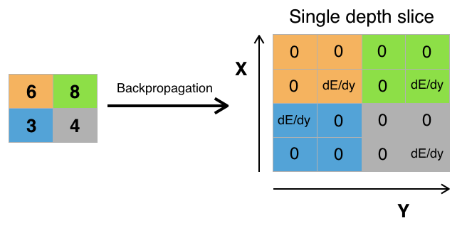
Backprop through Maxpooling

The error “passes” only through those values of the initial matrix that were chosen as the maximum at the max-cooling step. The remaining error values for the matrix will be zero (which is logical, because the values for these elements were not selected by the max-spooling function during the direct passage through the network and, accordingly, did not affect the final result).

Here is the python maxpooling implementation:

code_demo_maxpool.py

git link

import numpy as np y_l = np.array([ [1,0,2,3], [4,6,6,8], [3,1,1,0], [1,2,2,4]]) other_parameters={ 'convolution':False, 'stride':2, 'center_window':(0,0), 'window_shape':(2,2) } def maxpool(y_l, conv_params): indexes_a, indexes_b = create_indexes(size_axis=conv_params['window_shape'], center_w_l=conv_params['center_window']) stride = conv_params['stride'] #          y_l_mp = np.zeros((1,1)) #  y_l    y_l_mp_to_y_l = np.zeros((1,1), dtype='<U32') #   backprop    (    ) #          if conv_params['convolution']: g = 1 #   else: g = -1 #   #   i  j   y_l  ,        for i in range(y_l.shape[0]): for j in range(y_l.shape[1]): result = -np.inf element_exists = False for a in indexes_a: for b in indexes_b: # ,        if i*stride - g*a >= 0 and j*stride - g*b >= 0 \ and i*stride - g*a < y_l.shape[0] and j*stride - g*b < y_l.shape[1]: if y_l[i*stride - g*a][j*stride - g*b] > result: result = y_l[i*stride - g*a][j*stride - g*b] i_back = i*stride - g*a j_back = j*stride - g*b element_exists = True #       ,    i  j    if element_exists: if i >= y_l_mp.shape[0]: #  ,    y_l_mp = np.vstack((y_l_mp, np.zeros(y_l_mp.shape[1]))) #  y_l_mp_to_y_l    y_l_mp y_l_mp_to_y_l = np.vstack((y_l_mp_to_y_l, np.zeros(y_l_mp_to_y_l.shape[1]))) if j >= y_l_mp.shape[1]: #  ,    y_l_mp = np.hstack((y_l_mp, np.zeros((y_l_mp.shape[0],1)))) y_l_mp_to_y_l = np.hstack((y_l_mp_to_y_l, np.zeros((y_l_mp_to_y_l.shape[0],1)))) y_l_mp[i][j] = result #   y_l_mp_to_y_l   , #          y_l y_l_mp_to_y_l[i][j] = str(i_back) + ',' + str(j_back) return y_l_mp, y_l_mp_to_y_l def create_axis_indexes(size_axis, center_w_l): coordinates = [] for i in range(-center_w_l, size_axis-center_w_l): coordinates.append(i) return coordinates def create_indexes(size_axis, center_w_l): #              coordinates_a = create_axis_indexes(size_axis=size_axis[0], center_w_l=center_w_l[0]) coordinates_b = create_axis_indexes(size_axis=size_axis[1], center_w_l=center_w_l[1]) return coordinates_a, coordinates_b out_maxpooling = maxpool(y_l, other_parameters) print(' :', '\n', out_maxpooling[0]) print('\n', '    backprop:', '\n', out_maxpooling[1])

Sample script output

The second matrix that the function returns is the coordinates of the elements selected from the original matrix during the max-mining operation.

Backprop through a convolutional network

Displays backprop formula for convolution kernel update

\ begin {array} {rcl} \ dfrac {\ partial E} {\ partial w ^ l_ {ab}} & = & \ sum_ {i} \ sum_ {j} \ dfrac {\ partial E} {\ partial y ^ l_ {ij}} \ dfrac {\ partial y ^ l_ {ij}} {\ partial x ^ l_ {ij}} \ dfrac {\ partial x ^ l_ {ij}} {\ partial w ^ l_ {ab}} \\ & = & ^ {(1)} \ sum_ {i} \ sum_ {j} \ dfrac {\ partial E} {\ partial y ^ l_ {ij}} \ dfrac {\ partial y ^ l_ {ij}} {\ partial x ^ l_ {ij}} \ cdot \ dfrac {\ partial \ left (\ sum_ {a '= - \ infty} ^ {+ \ infty} \ sum_ {b' = - \ infty} ^ {+ \ infty} w ^ l_ {a'b '} \ cdot y ^ {l-1} _ {(is-a') (js-b ')} + b ^ l \ right)} {\ partial w ^ l_ { ab}} \\ & = & ^ {(2)} \ sum_ {i} \ sum_ {j} \ dfrac {\ partial E} {\ partial y ^ l_ {ij}} \ dfrac {\ partial y ^ l_ { ij}} {\ partial x ^ l_ {ij}} \ cdot y ^ {l-1} _ {(is-a) (js-b)} \\ && \ forall a \ in (- \ infty, .. ., + \ infty) \ enspace \ forall b \ in (- \ infty, ..., + \ infty) \ end {array}

$\ begin {array} {rcl} \ dfrac {\ partial E} {\ partial w ^ l_ {ab}} & = & \ sum_ {i} \ sum_ {j} \ dfrac {\ partial E} {\ partial y ^ l_ {ij}} \ dfrac {\ partial y ^ l_ {ij}} {\ partial x ^ l_ {ij}} \ dfrac {\ partial x ^ l_ {ij}} {\ partial w ^ l_ {ab}} \\ & = & ^ {(1)} \ sum_ {i} \ sum_ {j} \ dfrac {\ partial E} {\ partial y ^ l_ {ij}} \ dfrac {\ partial y ^ l_ {ij}} {\ partial x ^ l_ {ij}} \ cdot \ dfrac {\ partial \ left (\ sum_ {a '= - \ infty} ^ {+ \ infty} \ sum_ {b' = - \ infty} ^ {+ \ infty} w ^ l_ {a'b '} \ cdot y ^ {l-1} _ {(is-a') (js-b ')} + b ^ l \ right)} {\ partial w ^ l_ { ab}} \\ & = & ^ {(2)} \ sum_ {i} \ sum_ {j} \ dfrac {\ partial E} {\ partial y ^ l_ {ij}} \ dfrac {\ partial y ^ l_ { ij}} {\ partial x ^ l_ {ij}} \ cdot y ^ {l-1} _ {(is-a) (js-b)} \\ && \ forall a \ in (- \ infty, .. ., + \ infty) \ enspace \ forall b \ in (- \ infty, ..., + \ infty) \ end {array}$

(1) here we simply substitute the formula for

x_{i j}^{l}

$x ^ l_ {ij}$ strokes over

a^{'}

$a '$ and

b^{'}

$b '$ simply denote that this is another iterator.
(2) here we decompose the sum in the numerator by

a

$a$ and

b

$b$ :

s m a l l s u m_{i} s u m_{j} f r a c p a r t i a l E p a r t i a l y_{i j}^{l} f r a c p a r t i a l y_{i j}^{l} p a r t i a l x_{i j}^{l} f r a c p a r t i a l l e f t (w_{- i n f t y, - i n f t y}^{l} c d o t y_{(i s + i n f t y) (j s + i n f t y)}^{l - 1} + l d o t s + w_{a b}^{l} c d o t y_{(i s - a) (j s - b)}^{l - 1} + l d o t s + w_{i n f t y, i n f t y}^{l} c d o t y_{(i s - i n f t y) (j s - i n f t y)}^{l - 1} + b^{l} r i g h t) p a r t i a l w_{a b}^{l}

$\ small \ sum_ {i} \ sum_ {j} \ frac {\ partial E} {\ partial y ^ l_ {ij}} \ frac {\ partial y ^ l_ {ij}} {\ partial x ^ l_ {ij }} \ frac {\ partial \ left (w ^ l _ {- \ infty, - \ infty} \ cdot y ^ {l-1} _ {(is + \ infty) (js + \ infty)} + \ ldots + w ^ l_ {ab} \ cdot y ^ {l-1} _ {(is-a) (js-b)} + \ ldots + w ^ l _ {\ infty, \ infty} \ cdot y ^ {l-1} _ {(is- \ infty) (js- \ infty)} + b ^ l \ right)} {\ partial w ^ l_ {ab}}$

that is, all partial derivatives in the numerator, except those for which

a^{'} = a, b^{'} = b

$a '= a, b' = b$ will be zero. Wherein

l a r g e f r a c p a r t i a l w_{a b}^{l} c d o t y_{(i s - a) (j s - b)}^{l - 1} p a r t i a l w_{a b}^{l}

$\ large \ frac {\ partial w ^ l_ {ab} \ cdot y ^ {l-1} _ {(is-a) (js-b)}} {\ partial w ^ l_ {ab}}$ equals

y_{(i s - a) (j s - b)}^{l - 1}

$y ^ {l-1} _ {(is-a) (js-b)}$

All above refers to convolution. The backprop formula for cross-correlation is similar, except for the change of sign when

a

$a$ and

b

$b$ :

f r a c p a r t i a l E p a r t i a l w_{a b}^{l} = s u m_{i} s u m_{j} f r a c p a r t i a l E p a r t i a l y_{i j}^{l} f r a c p a r t i a l y_{i j}^{l} p a r t i a l x_{i j}^{l} c d o t y_{(i s + a) (j + b)}^{l - 1}

$\ frac {\ partial E} {\ partial w ^ l_ {ab}} = \ sum_ {i} \ sum_ {j} \ frac {\ partial E} {\ partial y ^ l_ {ij}} \ frac {\ partial y ^ l_ {ij}} {\ partial x ^ l_ {ij}} \ cdot y ^ {l-1} _ {(is + a) (j + b)}$

Here it is important to see that the convolution kernel itself does not participate in the final formula. There is a kind of convolution operation, but with the participation of

l a r g e f r a c p a r t i a l E p a r t i a l x_{i j}^{l}

$\ large \ frac {\ partial E} {\ partial x ^ l_ {ij}}$ and

y^{l - 1}

$y ^ {l-1}$ , with the role of the core

l a r g e f r a c p a r t i a l E p a r t i a l x_{i j}^{l}

$\ large \ frac {\ partial E} {\ partial x ^ l_ {ij}}$ , but still it is a little like convolution, especially with a step value greater than one: then

l a r g e f r a c p a r t i a l E p a r t i a l x_{i j}^{l}

$\ large \ frac {\ partial E} {\ partial x ^ l_ {ij}}$ “Splits” by

y^{l - 1}

$y ^ {l-1}$ that completely ceases to resemble familiar convolution. This “decay” is due to the fact that

i

$i$ and

j

$j$ iterated inside the formula loop. You can see how it all looks with the help of the demo code:

code_demo_convolution_back_dEdw_l.py

git link

 import numpy as np w_l_shape = (2,2) #  stride = 1 dEdx_l = np.array([ [1,2,3,4], [5,6,7,8], [9,10,11,12], [13,14,15,16]]) #  stride = 2  'convolution':False (   - x_l   ) # dEdx_l = np.array([ # [1,2], # [3,4]]) #  stride = 2  'convolution':True # dEdx_l = np.array([ # [1,2,3], # [4,5,6], # [7,8,9]]) y_l_minus_1 = np.zeros((4,4)) other_parameters={ 'convolution':True, 'stride':1, 'center_w_l':(0,0) } def convolution_back_dEdw_l(y_l_minus_1, w_l_shape, dEdx_l, conv_params): indexes_a, indexes_b = create_indexes(size_axis=w_l_shape, center_w_l=conv_params['center_w_l']) stride = conv_params['stride'] dEdw_l = np.zeros((w_l_shape[0], w_l_shape[1])) #          if conv_params['convolution']: g = 1 #   else: g = -1 #   #   a  b   for a in indexes_a: for b in indexes_b: #        y_l,         (  stride>1)  x_l demo = np.zeros([y_l_minus_1.shape[0], y_l_minus_1.shape[1]]) result = 0 for i in range(dEdx_l.shape[0]): for j in range(dEdx_l.shape[1]): # ,        if i*stride - g*a >= 0 and j*stride - g*b >= 0 \ and i*stride - g*a < y_l_minus_1.shape[0] and j*stride - g*b < y_l_minus_1.shape[1]: result += y_l_minus_1[i*stride - g*a][j*stride - g*b] * dEdx_l[i][j] demo[i*stride - g*a][j*stride - g*b] = dEdx_l[i][j] dEdw_l[indexes_a.index(a)][indexes_b.index(b)] = result #    ""      w_l #   demo     print('a=' + str(a) + '; b=' + str(b) + '\n', demo) return dEdw_l def create_axis_indexes(size_axis, center_w_l): coordinates = [] for i in range(-center_w_l, size_axis-center_w_l): coordinates.append(i) return coordinates def create_indexes(size_axis, center_w_l): #              coordinates_a = create_axis_indexes(size_axis=size_axis[0], center_w_l=center_w_l[0]) coordinates_b = create_axis_indexes(size_axis=size_axis[1], center_w_l=center_w_l[1]) return coordinates_a, coordinates_b print(convolution_back_dEdw_l(y_l_minus_1, w_l_shape, dEdx_l, other_parameters))

Sample script output

Displays the backprop formula for updating bias scales

Similar to the previous paragraph, only replace

w_{a b}^{l}

$w_ {ab} ^ l$ on

b^{l}

$b ^ l$ . We will use one bias for one feature map:

\ begin {array} {rcl} \ dfrac {\ partial E} {\ partial b ^ l} ​​& = & \ sum_ {i} \ sum_ {j} \ dfrac {\ partial E} {\ partial y ^ l_ { ij}} \ dfrac {\ partial y ^ l_ {ij}} {\ partial x ^ l_ {ij}} \ dfrac {\ partial x ^ l_ {ij}} {\ partial b ^ l} ​​\\ & = & \ small \ sum_ {i} \ sum_ {j} \ dfrac {\ partial E} {\ partial y ^ l_ {ij}} \ dfrac {\ partial y ^ l_ {ij}} {\ partial x ^ l_ {ij}} \ cdot \ dfrac {\ partial \ left (\ sum_ {a = - \ infty} ^ {+ \ infty} \ sum_ {b = - \ infty} ^ {+ \ infty} w ^ l_ {ab} \ cdot y ^ {l-1} _ {(is-a) (js-b)} + b ^ l \ right)} {\ partial b ^ l} ​​\\ & = & \ sum_ {i} \ sum_ {j} \ dfrac {\ partial E} {\ partial y ^ l_ {ij}} \ dfrac {\ partial y ^ l_ {ij}} {\ partial x ^ l_ {ij}} \ end {array}

$\ begin {array} {rcl} \ dfrac {\ partial E} {\ partial b ^ l} & = & \ sum_ {i} \ sum_ {j} \ dfrac {\ partial E} {\ partial y ^ l_ { ij}} \ dfrac {\ partial y ^ l_ {ij}} {\ partial x ^ l_ {ij}} \ dfrac {\ partial x ^ l_ {ij}} {\ partial b ^ l} \\ & = & \ small \ sum_ {i} \ sum_ {j} \ dfrac {\ partial E} {\ partial y ^ l_ {ij}} \ dfrac {\ partial y ^ l_ {ij}} {\ partial x ^ l_ {ij}} \ cdot \ dfrac {\ partial \ left (\ sum_ {a = - \ infty} ^ {+ \ infty} \ sum_ {b = - \ infty} ^ {+ \ infty} w ^ l_ {ab} \ cdot y ^ {l-1} _ {(is-a) (js-b)} + b ^ l \ right)} {\ partial b ^ l} \\ & = & \ sum_ {i} \ sum_ {j} \ dfrac {\ partial E} {\ partial y ^ l_ {ij}} \ dfrac {\ partial y ^ l_ {ij}} {\ partial x ^ l_ {ij}} \ end {array}$

that is, if you decompose the sum over all

i

$i$ and

j

$j$ , we will see that all partial derivatives by

p a r t i a l b^{l}

$\ partial b ^ l$ will be equal to one:

f r a c p a r t i a l l e f t (s u m_{a = - i n f t y}^{+ i n f t y} s u m_{b = - i n f t y}^{+ i n f t y} w_{a b}^{l} c d o t y_{(i s - a) (j s - b)}^{l - 1} + b^{l} r i g h t) p a r t i a l b^{l} ​ ​ = 1

$\ frac {\ partial \ left (\ sum_ {a = - \ infty} ^ {+ \ infty} \ sum_ {b = - \ infty} ^ {+ \ infty} w ^ l_ {ab} \ cdot y ^ { l-1} _ {(is-a) (js-b)} + b ^ l \ right)} {\ partial b ^ l} = 1$

For one feature map, there is only one bias that is “associated” with all the elements of this map. Accordingly, when adjusting the bias value, all the values from the map obtained during back propagation of the error should be taken into account. As an alternative, you can take as many bias for a separate feature map as there are elements in this map, but in this case, the bias parameters are too many — more than the parameters of the convolution kernels themselves. For the second case it is also easy to calculate the derivative - then each

l a r g e f r a c p a r t i a l E p a r t i a l b_{i j}^{l}

$\ large \ frac {\ partial E} {\ partial b ^ l_ {ij}}$ (note bias has already had subscripts

i j

$ij$ ) will be equal to each

l a r g e f r a c p a r t i a l E p a r t i a l x_{i j}^{l}

$\ large \ frac {\ partial E} {\ partial x ^ l_ {ij}}$ .

Derivation of the backprop formula through the convolution layer

Here, everything is similar to the previous conclusions:

\ begin {array} {rcl} \ dfrac {\ partial E} {\ partial y ^ {l-1} _ {ij}} & = & \ sum_ {i '} \ sum_ {j'} \ dfrac {\ partial E} {\ partial y ^ l_ {i'j '}} \ dfrac {\ partial y ^ l_ {i'j'}} {\ partial x ^ l_ {i'j '}} \ dfrac {\ partial x ^ l_ {i'j '}} {\ partial y ^ {l-1} _ {ij}} \\ & = & \ sum_ {i'} \ sum_ {j '} \ dfrac {\ partial E} {\ partial y ^ l_ {i'j '}} \ dfrac {\ partial y ^ l_ {i'j'}} {\ partial x ^ l_ {i'j '}} \ cdot \ dfrac {\ partial \ left (\ sum_ {a = - \ infty} ^ {+ \ infty} \ sum_ {b = - \ infty} ^ {+ \ infty} w ^ l_ {ab} \ cdot y ^ {l-1} _ {(i's-a ) (j's-b)} + b ^ l \ right)} {\ partial y ^ {l-1} _ {ij}} \\ & = & \ sum_ {i '} \ sum_ {j'} \ dfrac { \ partial E} {\ partial y ^ l_ {i'j '}} \ dfrac {\ partial y ^ l_ {i'j'}} {\ partial x ^ l_ {i'j '}} \ cdot w ^ { l} _ {(i's-i) (j's-j)} \\ && \ forall i, j \ in dimension \ enspace of matrix \ enspace y ^ {l-1} \ end {array}

$\ begin {array} {rcl} \ dfrac {\ partial E} {\ partial y ^ {l-1} _ {ij}} & = & \ sum_ {i '} \ sum_ {j'} \ dfrac {\ partial E} {\ partial y ^ l_ {i'j '}} \ dfrac {\ partial y ^ l_ {i'j'}} {\ partial x ^ l_ {i'j '}} \ dfrac {\ partial x ^ l_ {i'j '}} {\ partial y ^ {l-1} _ {ij}} \\ & = & \ sum_ {i'} \ sum_ {j '} \ dfrac {\ partial E} {\ partial y ^ l_ {i'j '}} \ dfrac {\ partial y ^ l_ {i'j'}} {\ partial x ^ l_ {i'j '}} \ cdot \ dfrac {\ partial \ left (\ sum_ {a = - \ infty} ^ {+ \ infty} \ sum_ {b = - \ infty} ^ {+ \ infty} w ^ l_ {ab} \ cdot y ^ {l-1} _ {(i's-a ) (j's-b)} + b ^ l \ right)} {\ partial y ^ {l-1} _ {ij}} \\ & = & \ sum_ {i '} \ sum_ {j'} \ dfrac { \ partial E} {\ partial y ^ l_ {i'j '}} \ dfrac {\ partial y ^ l_ {i'j'}} {\ partial x ^ l_ {i'j '}} \ cdot w ^ { l} _ {(i's-i) (j's-j)} \\ && \ forall i, j \ in dimension \ enspace of matrix \ enspace y ^ {l-1} \ end {array}$

Decomposing the sum in numerator by

a

$a$ and

b

$b$ , we obtain that all partial derivatives are equal to zero, except in the case when

i^{'} s - a = i

$i's-a = i$ and

j^{'} s - b = j

$j's-b = j$ , and correspondingly,

a = i^{'} s - i

$a = i's-i$ ,

b = j^{'} s - j

$b = j's-j$ . This is true only for convolution, for cross-correlation there should be

i^{'} s + a = i

$i's + a = i$ and

j^{'} s + b = j

$j's + b = j$ and correspondingly,

a = i - i^{'} s

$a = i-i's$ and

b = j - j^{'} s

$b = j-j's$ . And then the final formula in the case of cross-correlation will look like this:

f r a c p a r t i a l E p a r t i a l y_{i j}^{l - 1} = s u m_{i^{'}} s u m_{j^{'}} f r a c p a r t i a l E p a r t i a l y_{i^{'} j^{'}}^{l} f r a c p a r t i a l y_{i^{'} j^{'}}^{l} p a r t i a l x_{i^{'} j^{'}}^{l} c d o t w_{(i - i^{'} s) (j - j^{'} s)}^{l}

$\ frac {\ partial E} {\ partial y ^ {l-1} _ {ij}} = \ sum_ {i '} \ sum_ {j'} \ frac {\ partial E} {\ partial y ^ l_ { i'j '}} \ frac {\ partial y ^ l_ {i'j'}} {\ partial x ^ l_ {i'j '}} \ cdot w ^ {l} _ {(i-i's) (j -j's)}$

The resulting expressions are the same convolution operation, with the familiar kernel being the core.

w^{l}

$w ^ l$ . But, the truth is, everything looks like a familiar convolution only if stride is equal to one, in cases of another step, something completely different is already obtained (similar to the case of backprop for updating the convolution kernel): matrix

w^{l}

$w ^ l$ starts to “break” across the matrix

l a r g e f r a c p a r t i a l E p a r t i a l x^{l} ​ ​

$\ large \ frac {\ partial E} {\ partial x ^ l} $ , capturing its different parts (again, because the indices

i^{'}

$i '$ and

j^{'}

$j '$ at

w^{l}

$w ^ l$ iterated inside the formula loop).

Here you can see and test the code:

code_demo_convolution_back_dEdy_l_minus_1.py

git link

 import numpy as np w_l = np.array([ [1,2], [3,4]]) #  stride = 1 dEdx_l = np.zeros((3,3)) #  stride = 2  'convolution':False (   - x_l    ) # dEdx_l = np.zeros((2,2)) #  stride = 2  'convolution':True # dEdx_l = np.zeros((2,2)) y_l_minus_1_shape = (3,3) other_parameters={ 'convolution':True, 'stride':1, 'center_w_l':(0,0) } def convolution_back_dEdy_l_minus_1(dEdx_l, w_l, y_l_minus_1_shape, conv_params): indexes_a, indexes_b = create_indexes(size_axis=w_l.shape, center_w_l=conv_params['center_w_l']) stride = conv_params['stride'] dEdy_l_minus_1 = np.zeros((y_l_minus_1_shape[0], y_l_minus_1_shape[1])) #          if conv_params['convolution']: g = 1 #   else: g = -1 #   for i in range(dEdy_l_minus_1.shape[0]): for j in range(dEdy_l_minus_1.shape[1]): result = 0 #     demo = np.zeros([dEdx_l.shape[0], dEdx_l.shape[1]]) for i_x_l in range(dEdx_l.shape[0]): for j_x_l in range(dEdx_l.shape[1]): #    ""      w_l a = g*i_x_l*stride - g*i b = g*j_x_l*stride - g*j #         if a in indexes_a and b in indexes_b: a = indexes_a.index(a) b = indexes_b.index(b) result += dEdx_l[i_x_l][j_x_l] * w_l[a][b] demo[i_x_l][j_x_l] = w_l[a][b] dEdy_l_minus_1[i][j] = result #   demo     print('i=' + str(i) + '; j=' + str(j) + '\n', demo) return dEdy_l_minus_1 def create_axis_indexes(size_axis, center_w_l): coordinates = [] for i in range(-center_w_l, size_axis-center_w_l): coordinates.append(i) return coordinates def create_indexes(size_axis, center_w_l): #              coordinates_a = create_axis_indexes(size_axis=size_axis[0], center_w_l=center_w_l[0]) coordinates_b = create_axis_indexes(size_axis=size_axis[1], center_w_l=center_w_l[1]) return coordinates_a, coordinates_b print(convolution_back_dEdy_l_minus_1(dEdx_l, w_l, y_l_minus_1_shape, other_parameters))

Sample script output

Interestingly, if we perform cross-correlation, then at the stage of direct passage through the network, we do not turn the convolution kernel upside down, but we turn it over during the back propagation of the error when passing through the convolution layer. If we apply the convolution formula, everything happens exactly the opposite.

In this article, we have deduced and examined in detail all the formulas for the back-propagation of error, that is, formulas that allow the future model to be trained. In the next article, we will connect all this into one integral code, which will be called a convolutional network, and we will try to train this network to predict classes on a real dataset. And also we will check, how much all calculations are correct in comparison with the library for machine learning tensorflow.

Source: https://habr.com/ru/post/344116/

All Articles

Convolution network in python. Part 2. Derivation of formulas for training models

Derivation of a formula for back propagation of an error through the loss function

Output backprop formula through activation functions

... via ReLU

... through sigmoid

... also via softmax (or here )

Backprop through a full mesh network

Displaying the backprop formula for updating the weights matrix wl w ^ l fc networks

Displaying the backprop formula to update the matrix bl b ^ {l}

The output of the formula is backprop through yl−1 y ^ {l-1}

Backprop through Maxpooling

Backprop through a convolutional network

Displays backprop formula for convolution kernel update

Displays the backprop formula for updating bias scales

Derivation of the backprop formula through the convolution layer

More articles:

Displaying the backprop formula for updating the weights matrix $w ^ l$ fc networks

Displaying the backprop formula to update the matrix $b ^ {l}$

The output of the formula is backprop through $y ^ {l-1}$