Convolution network in python. Part 1. Determination of the basic parameters of the model

Despite the fact that more than one article can be found explaining the principle of the method of back-propagation of error in convolutional networks ( one , two , three , four , five, and even giving an “intuitive” understanding - six ), I, nevertheless, did not succeed fully understand this topic. It seems that the authors do not pay enough attention to the usual examples, or else they omit some features that are well understood by them, but not obvious to others, and all the material for this reason becomes overwhelming. I wanted to sort it all out for myself and as a result, the notes turned into an article. I tried to eliminate all the shortcomings of the existing explanations and I hope that this article will not cause any questions or misunderstandings to anyone. And maybe the next newcomer, who, like me, wants to figure everything out, will spend less time already.

In this first article, we will look at the architecture of the future network, and all the formulas for direct passage through this network. In the second article we will dwell on the back propagation of the error, derive and analyze the formulas - for the sake of this part everything was started, it was the formulas for training the model and especially the convolutional layer that seemed to me the most difficult. The last article will present an approximate view of the network implementation in python, and also try to train the network in real dataset and compare the results with the same implementation, but using the tensorflow library. During the whole material I will lay out the python code in parts so that you can immediately see the implementation of the formulas. When writing the code, I focused on the fact that the formulas are easy to “read” in the lines, less time is spent on optimization and beauty. In general, the ultimate goal is for the reader to understand all the subtleties of updating the parameters of a convolutional and fully connected network and to be able to imagine what the working code of this network might look like.

What will not be in these articles? Explanations of the foundations of mathematics and partial derivatives, details of the “intuitive” understanding of the essence of backpropagation (you can read this excellent article for a start) or how networks work in general, including convolutional networks. For a better understanding of the material, it is desirable to know these things and especially the basics of the work of neural networks.
So, the first article.

Convolution

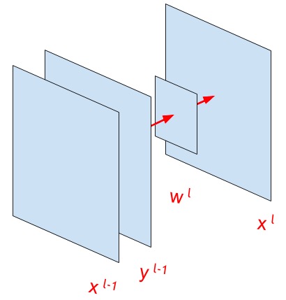
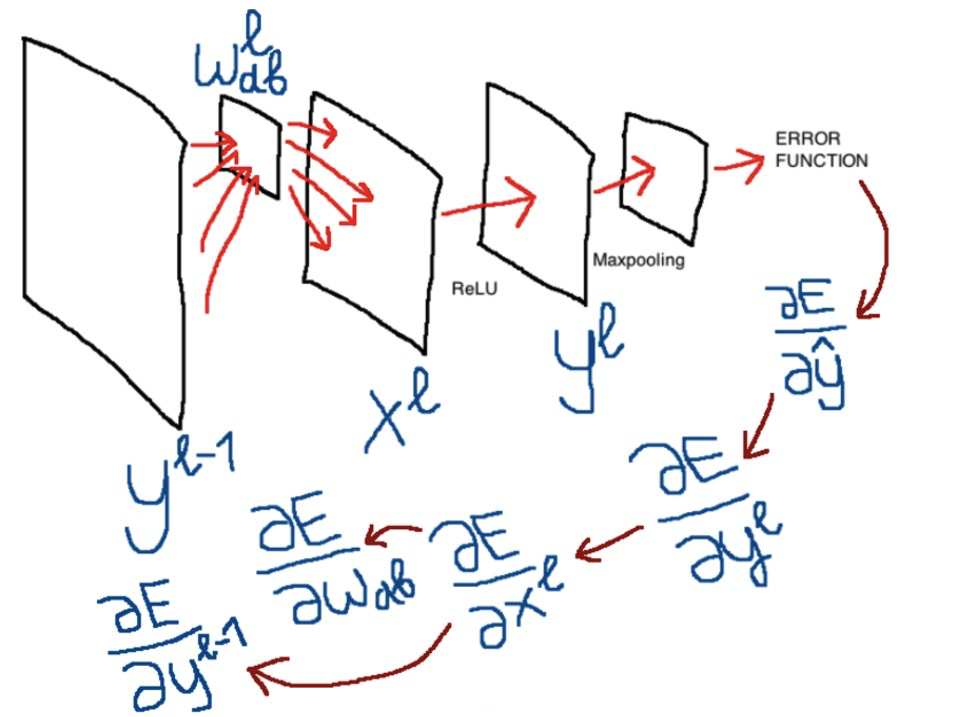
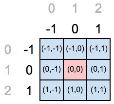
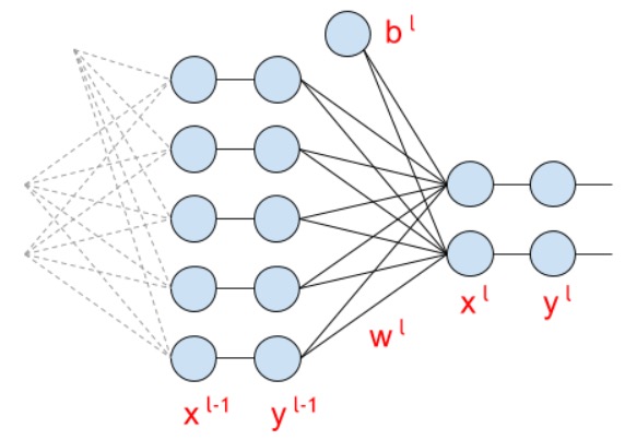
The illustration above indicates the main variables that will be used in the following.
')
Let's look at the convolution formula. But first, what do we want to see in the formula, what should it reflect? Let's turn to Wikipedia :

“In the convolutional neural network, only a limited matrix of small weights is used in the convolution operation, which is“ moved ”across the entire processed layer (at the very beginning, directly in the input image), forming an activation signal for the neuron of the next layer with a similar position after each shift. That is, for different neurons of the output layer, the same weights matrix is used, which is also called the convolution kernel ... Then the next layer resulting from the convolution operation with such weights matrix shows the presence of this feature in the processed layer and its coordinates, forming the so-called feature map (English feature map). ”

So the convolution formula should show the “motion” of the nucleus.

w^{l}

$w ^ l$ by input image or feature map

y^{l - 1}

$y ^ {l-1}$ . This is what the following formula shows:

x_{i j}^{l} = s u m_{a = - i n f t y}^{+ i n f t y} s u m_{b = - i n f t y}^{+ i n f t y} w_{a b}^{l} c d o t y_{(i c d o t s a) (j c d o t s b)}^{l - 1} + b^{l} q q u a d f o r a l l i i n (0, . . ., N) e n s p a c e f o r a l l j i n (0, . . ., M)

$x ^ l_ {ij} = \ sum_ {a = - \ infty} ^ {+ \ infty} \ sum_ {b = - \ infty} ^ {+ \ infty} w ^ l_ {ab} \ cdot y ^ {l -1} _ {(i \ cdot sa) (j \ cdot sb)} + b ^ l \ qquad \ forall i \ in (0, ..., N) \ enspace \ forall j \ in (0, .. ., M)$

Here subscripts

i

$i$ ,

j

$j$ ,

a

$a$ ,

b

$b$ Are the indices of the elements in the matrices, and

s

$s$ - the size of the step of convolution (stride).

Superscripts

l

$l$ and

l - 1

$l-1$ - These are indices of network layers.

x^{l - 1}

$x ^ {l-1}$ - the output of some previous function, or the input image of the network

y^{l - 1}

$y ^ {l-1}$ - this

x^{l - 1}

$x ^ {l-1}$ after passing the activation function (for example, relu or sigmoid; the item about the activation function will be a little later)

w^{l}

$w ^ l$ - convolution kernel

b^{l}

$b ^ l$ - bias or offset (absent in the picture above)

x^{l}

$x ^ l$ - The result of the operation of convolution. That is, operations take place separately for each element.

i j

$ij$ matrices

x^{l}

$x ^ l$ whose dimension

(N, M)

$(N, M)$ .

Below is an excellent illustration of the work of the convolution formula Blue is displayed

y^{l - 1}

$y ^ {l-1}$ , green -

x^{l}

$x ^ l$ and a three-by-three gray moving matrix is the convolution kernel

w^{l}

$w ^ l$ :

Having dealt with the parameter designations and understanding the basic principle of the convolution operation (the details of the convolution formula will become clear towards the end of the article, so you may need to come back here later), you can go on to the important nuance of this formula and the operation itself: the core has a central element . Moreover, the central element may not necessarily be in the center (where is the center of the matrix two by two pixels?), But in general in any cell of the core - which one you want. For example, the central element of the kernel in the animation above is at position (1.1), and the relative convolution operation of this element occurs. So, what is the central element?

Central element of the core

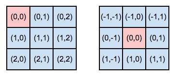
So, the indexing of core elements occurs depending on the location of the central element. In fact, the central element defines the beginning of the “coordinate axis” of the convolution kernel. Look at the picture below, on the left, the core with the central element in the zero row and zero column, on the right - in the first row and first column:

See how indexing has changed? And yes, I say that in the second core, the central element “moved” to the first row of the first column, meaning that this happened relative to the numbering of the first core. In fact, the indices of the central element are always equal (0,0), and for convenience of further exposition, I will say the “old” coordinates, speaking of the position of the central element in the upper left corner, and the “new” coordinates - about the position of the central element in any elsewhere in the kernel, using the numbering of the “old” coordinate grid (for example, (1,1) for the right convolution kernel in the figure above).

But, going back to the convolution formula, what does it mean - the sum from minus infinity to plus infinity? After all, the core itself has quite specific dimensions and it does not have an infinite number of elements. I found different spellings of the formula, for example,

s u m_{u = - a}^{a} s u m_{v = - b}^{b}

$\ sum_ {u = -a} ^ {a} \ sum_ {v = -b} ^ {b}$ ( here and here ). I also found variants with infinity, as in the variant at the beginning of the article ( here and here ). But the latter seemed to me a more “common” case.

The minus in the convolution kernel formula is a consequence of the location of the central element. We should “go through” all possible existing elements, and we can start from minus infinity. Or from minus

a

$a$ and

b

$b$ . If an element by these indices is not defined for a given kernel, then multiplication occurs by zero, and in fact operations start not from minus infinity, but from the position of the central element multiplied by minus one (in the numbering of the “old” coordinates). And the operation will end not at plus infinity, but at the difference between the number of core elements along the axis under consideration minus the index of the central element (again, in the numbering of the “old” coordinate axis). And the last value of the resulting range is not included (since the indexation is from zero).

In words, it may sound hard, and probably best to see how this can be done in python. Below is the code for calculating the indices for the “new” axis of the core, depending on the selected central element:

code_demo_indexes.py

git link

import numpy as np size_axis = (3,3) center_w_l = (1,1) def create_axis_indexes(size_axis, center_w_l): coordinates = [] for i in range(-center_w_l, size_axis-center_w_l): coordinates.append(i) return coordinates def create_indexes(size_axis, center_w_l): #              coordinates_a = create_axis_indexes(size_axis=size_axis[0], center_w_l=center_w_l[0]) coordinates_b = create_axis_indexes(size_axis=size_axis[1], center_w_l=center_w_l[1]) return coordinates_a, coordinates_b print(create_indexes(size_axis, center_w_l))

In the picture below, we declared the element in position (1,1) as the center of the core.

But the “old” coordinates tell us that the position of the central element must be in indices (0,0), which means that it is necessary to redefine the coordinate axes for the new position of the central element.

If we substitute our values into the code above, we will get the filled Python list with values from range (-1, 2), that is, the list will contain [-1,0,1]. Once again, why range (-1, 2)? “Minus one” because the operation starts from the minus index of our central element, and “two” is obtained as the axis length (equal to three) minus the index of the central element in the old coordinates (that is, one). The last element of the range is not included.

Cross correlation

I will cite once again the convolution formula:

x_{i j}^{l} = s u m_{a = - i n f t y}^{+ i n f t y} s u m_{b = - i n f t y}^{+ i n f t y} w_{a b}^{l} c d o t y_{(i c d o t s a) (j c d o t s b)}^{l - 1} + b^{l} q q u a d f o r a l l i i n (0, . . ., N) e n s p a c e f o r a l l j i n (0, . . ., M)

And below is the cross-correlation formula:

x_{i j}^{l} = s u m_{a = - i n f t y}^{+ i n f t y} s u m_{b = - i n f t y}^{+ i n f t y} w_{a b}^{l} c d o t y_{(i c d o t s + a) (j c d o t s + b)}^{l - 1} + b^{l}

$x ^ l_ {ij} = \ sum_ {a = - \ infty} ^ {+ \ infty} \ sum_ {b = - \ infty} ^ {+ \ infty} w ^ l_ {ab} \ cdot y ^ {l -1} _ {(i \ cdot s + a) (j \ cdot s + b)} + b ^ l$

Yes, the only difference is that cons in the calculation of subscripts

y^{l - 1}

$y ^ {l-1}$ replaced by pluses. In practice, applying the convolution formula, we can see that the kernel “rolls over” during convolution (and overturns relative to the central element!), While at cross-correlation, the kernel elements retain their positions during the convolution. Look at the illustration to better understand what is meant here:

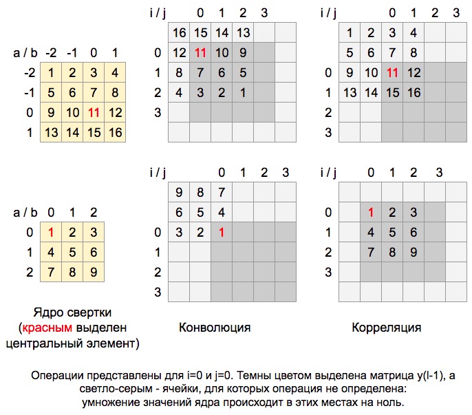
Here you can see the position of the kernel, its location during convolution relative to the matrix

y^{l - 1}

$y ^ {l-1}$ . Below is the code that also displays demo examples similar to those in the picture above, only for all

i

$i$ and

j

$j$

code_demo_convolution_feed_x_l.py

git link

 import numpy as np # w_l = np.array([ # [1,2,3,4], # [5,6,7,8], # [9,10,11,12], # [13,14,15,16]]) w_l = np.array([ [1,2], [3,4]]) y_l_minus_1 = np.zeros((3,3)) other_parameters={ 'convolution':True, 'stride':1, 'center_w_l':(0,0) } def convolution_feed_x_l(y_l_minus_1, w_l, conv_params): indexes_a, indexes_b = create_indexes(size_axis=w_l.shape, center_w_l=conv_params['center_w_l']) stride = conv_params['stride'] #          x_l = np.zeros((1,1)) #          if conv_params['convolution']: g = 1 #   else: g = -1 #   #   i  j   y_l_minus_1  ,     x_l    for i in range(y_l_minus_1.shape[0]): for j in range(y_l_minus_1.shape[1]): demo = np.zeros([y_l_minus_1.shape[0], y_l_minus_1.shape[1]]) #     result = 0 element_exists = False for a in indexes_a: for b in indexes_b: # ,        if i*stride - g*a >= 0 and j*stride - g*b >= 0 \ and i*stride - g*a < y_l_minus_1.shape[0] and j*stride - g*b < y_l_minus_1.shape[1]: result += y_l_minus_1[i*stride - g*a][j*stride - g*b] * w_l[indexes_a.index(a)][indexes_b.index(b)] #    ""      w_l demo[i*stride - g*a][j*stride - g*b] = w_l[indexes_a.index(a)][indexes_b.index(b)] element_exists = True #       ,    i  j    if element_exists: if i >= x_l.shape[0]: #  ,    x_l = np.vstack((x_l, np.zeros(x_l.shape[1]))) if j >= x_l.shape[1]: #  ,    x_l = np.hstack((x_l, np.zeros((x_l.shape[0],1)))) x_l[i][j] = result #   demo     print('i=' + str(i) + '; j=' + str(j) + '\n', demo) return x_l def create_axis_indexes(size_axis, center_w_l): coordinates = [] for i in range(-center_w_l, size_axis-center_w_l): coordinates.append(i) return coordinates def create_indexes(size_axis, center_w_l): #              coordinates_a = create_axis_indexes(size_axis=size_axis[0], center_w_l=center_w_l[0]) coordinates_b = create_axis_indexes(size_axis=size_axis[1], center_w_l=center_w_l[1]) return coordinates_a, coordinates_b print(convolution_feed_x_l(y_l_minus_1, w_l, other_parameters))

Sample script output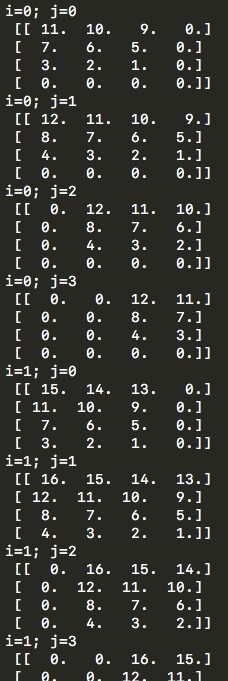

And I would immediately like to note that the choice of the central element or the convolution step size, the dimensions of the kernel matrix, the correlation or convolution formula — all these nuances are directly reflected in the backpropagation error formulas and therefore the training will take place correctly regardless of the selected parameters. In the code I tried to implement all these things, they can be customized and try to run everything yourself.

Depending on the convolution method - convolution or cross-correlation, different step sizes and the choice of the central core element - the dimension of the output matrix

x^{l}

$x ^ l$ may vary. In the simplest case, with a step equal to one, the dimension of the matrix

x^{l}

$x ^ l$ will be equal to the matrix

y^{l - 1}

$y ^ {l-1}$ . I am sure that the general formula for finding this dimension, that is, exactly the values

(N, M)

$(N, M)$ , taking into account all the listed features, it exists (see, for example, the documentation of tensorflow , but it only takes into account the possibility of different step sizes), but in the above function in python, initially the dimension of the matrix

x^{l}

$x ^ l$ not set, and rows and columns are added to this matrix as calculations are performed, which, of course, is not the optimal solution.

Activation functions

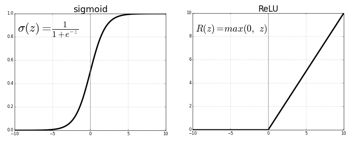
Below are the formulas of activation functions that can be used in a future model. In fact, this is just a “transformation”

x^{l}

$x ^ l$ at

y^{l}

$y ^ l$ in this way:

y^{l} = f (x^{l})

$y ^ l = f (x ^ l)$ . The activation function allows you to make the network non-linear , and if we did not use the activation functions (then it would turn out that

y^{l} = x^{l}

$y ^ l = x ^ l$ ) or would use a linear function, then it does not matter how many layers there would be in the network: they could all be replaced with a single layer with a linear activation function.

So, ReLU:

f_{R e L U} = m a x (0, x)

$f_ {ReLU} = max (0, x)$

And sigmoid:

f_{s i g m o i d} = f r a c 1 1 + e^{- x}

$f_ {sigmoid} = \ frac {1} {1 + e ^ {- x}}$

A sigmoid is used only if there are no more than two classes (for the classification task): the output of the model will be a number from zero (first class) to one (second class). For a larger number of classes, in order for the model output to reflect the probability of these classes (and the sum of the probabilities over the network outputs equals one), softmax is used. The function looks simple, but there will be certain difficulties in calculating the formula for backprop.

f_{s o f t m a x} = y_{i}^{l} = f (x_{i}^{l}) = f r a c e^{x_{i}^{l}} s u m_{k = 0}^{n} e^{x_{k}^{l}}

$f_ {softmax} = y ^ l_i = f (x ^ l_i) = \ frac {e ^ {x ^ l_i}} {\ sum_ {k = 0} ^ {n} e ^ {x ^ l_k}}$

Where

n

$n$ - this is the number of classes.

Makspool layer

This layer allows you to highlight important features on feature maps, gives invariance to finding an object on maps, and also reduces the dimensionality of maps, speeding up the network operation time.

Implementing maxpooling in python:

code_demo_maxpool.py

git link

 import numpy as np y_l = np.array([ [1,0,2,3], [4,6,6,8], [3,1,1,0], [1,2,2,4]]) other_parameters={ 'convolution':False, 'stride':2, 'center_window':(0,0), 'window_shape':(2,2) } def maxpool(y_l, conv_params): indexes_a, indexes_b = create_indexes(size_axis=conv_params['window_shape'], center_w_l=conv_params['center_window']) stride = conv_params['stride'] #          y_l_mp = np.zeros((1,1)) #  y_l    y_l_mp_to_y_l = np.zeros((1,1), dtype='<U32') #   backprop    (    ) #          if conv_params['convolution']: g = 1 #   else: g = -1 #   #   i  j   y_l  ,        for i in range(y_l.shape[0]): for j in range(y_l.shape[1]): result = -np.inf element_exists = False for a in indexes_a: for b in indexes_b: # ,        if i*stride - g*a >= 0 and j*stride - g*b >= 0 \ and i*stride - g*a < y_l.shape[0] and j*stride - g*b < y_l.shape[1]: if y_l[i*stride - g*a][j*stride - g*b] > result: result = y_l[i*stride - g*a][j*stride - g*b] i_back = i*stride - g*a j_back = j*stride - g*b element_exists = True #       ,    i  j    if element_exists: if i >= y_l_mp.shape[0]: #  ,    y_l_mp = np.vstack((y_l_mp, np.zeros(y_l_mp.shape[1]))) #  y_l_mp_to_y_l    y_l_mp y_l_mp_to_y_l = np.vstack((y_l_mp_to_y_l, np.zeros(y_l_mp_to_y_l.shape[1]))) if j >= y_l_mp.shape[1]: #  ,    y_l_mp = np.hstack((y_l_mp, np.zeros((y_l_mp.shape[0],1)))) y_l_mp_to_y_l = np.hstack((y_l_mp_to_y_l, np.zeros((y_l_mp_to_y_l.shape[0],1)))) y_l_mp[i][j] = result #   y_l_mp_to_y_l   , #          y_l y_l_mp_to_y_l[i][j] = str(i_back) + ',' + str(j_back) return y_l_mp, y_l_mp_to_y_l def create_axis_indexes(size_axis, center_w_l): coordinates = [] for i in range(-center_w_l, size_axis-center_w_l): coordinates.append(i) return coordinates def create_indexes(size_axis, center_w_l): #              coordinates_a = create_axis_indexes(size_axis=size_axis[0], center_w_l=center_w_l[0]) coordinates_b = create_axis_indexes(size_axis=size_axis[1], center_w_l=center_w_l[1]) return coordinates_a, coordinates_b out_maxpooling = maxpool(y_l, other_parameters) print(' :', '\n', out_maxpooling[0]) print('\n', '    backprop:', '\n', out_maxpooling[1])

Sample script output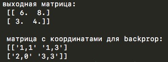

The code is very similar to the convolution function above, and even the same parameters are preserved: the choice of the strike, the flag of the operation of convolution or cross-correlation (since, according to the logic of this function, the max-scanning window is identical to the convolution kernel) and the choice of the central element. But, of course, here there is no element-by-element multiplication of matrices, but only, in fact, the choice of the maximum value from the specified window. The “classic” values of the max-cooling parameters in the convolution parameters are the cross-correlation and the position of the central element in the upper left corner.

The function from the demo code returns two matrices — an output matrix of a lower dimension and another matrix with the coordinates of the elements that were chosen as the maximum from the original matrix during the max-mining operation. The second matrix is useful during back propagation of an error.

Mesh network layer

After the layers of convolution, we get a set of feature maps. We will connect them into one vector and this vector will be fed to the input of a fully connected network.

The formula for the fc-layer (fully connected) looks like this:

x_{i}^{l} = s u m_{k = 0}^{m} w_{k i}^{l} y_{k}^{l - 1} + b_{i}^{l} q q u a d f o r a l l i i n (0, . . ., n)

$x ^ l_i = \ sum_ {k = 0} ^ {m} w ^ l_ {ki} y ^ {l-1} _k + b ^ l_i \ qquad \ forall i \ in (0, ..., n)$

And in the matrix view (under the line I wrote the dimensions of the matrices):

X^{l} = Y^{l - 1} W^{l} + B_{i}^{l} t i n y (1 t i m e s n) q u a d (1 t i m e s m) (m t i m e s n) q u a d (1 t i m e s n)

$X ^ l = Y ^ {l-1} W ^ l + B ^ l_i \\ \ tiny (1 \ times n) \ quad (1 \ times m) (m \ times n) \ quad (1 \ times n )$

And this is how these matrices look like during calculations:

\ begin {aligned} \ begin {bmatrix} & x ^ {l} _0 & x ^ {l} _1 & x ^ {l} _2 & ... & x ^ {l} _n \ end {bmatrix} = \ begin {bmatrix} & y ^ {l-1} _0 & y ^ {l-1} _1 & ... & y ^ {l-1} _m \ end {bmatrix} \ begin {bmatrix} & w ^ {l } _ {00} & w ^ {l} _ {01} & ... & w ^ {l} _ {0n} \\ & w ^ {l} _ {10} & w ^ {l} _ {11 } & ... & w ^ {l} _ {1n} \\ & ... & ... & ... & ... \\ & w ^ {l} _ {m0} & w ^ {l } _ {m1} & ... & w ^ {l} _ {mn} \ end {bmatrix} \\ \\ + \ begin {bmatrix} & b ^ {l} _0 & b ^ {l} _1 &. .. & b ^ {l} _n \ end {bmatrix} \ end {aligned}

$\ begin {aligned} \ begin {bmatrix} & x ^ {l} _0 & x ^ {l} _1 & x ^ {l} _2 & ... & x ^ {l} _n \ end {bmatrix} = \ begin {bmatrix} & y ^ {l-1} _0 & y ^ {l-1} _1 & ... & y ^ {l-1} _m \ end {bmatrix} \ begin {bmatrix} & w ^ {l } _ {00} & w ^ {l} _ {01} & ... & w ^ {l} _ {0n} \\ & w ^ {l} _ {10} & w ^ {l} _ {11 } & ... & w ^ {l} _ {1n} \\ & ... & ... & ... & ... \\ & w ^ {l} _ {m0} & w ^ {l } _ {m1} & ... & w ^ {l} _ {mn} \ end {bmatrix} \\ \\ + \ begin {bmatrix} & b ^ {l} _0 & b ^ {l} _1 &. .. & b ^ {l} _n \ end {bmatrix} \ end {aligned}$

Loss function

The final stage of the network is a function that assesses the quality of work of the entire model. The loss function is at the very end, after all layers of the network. It can look like this:

E = s u m_{i = 0}^{n} f r a c 12 (y_{i}^{t r u t h} - y_{i}^{l})^{2}

$E = \ sum_ {i = 0} ^ {n} \ frac {1} {2} (y ^ {truth} _i-y ^ l_i) ^ 2$

Where

n

$n$ Is the number of classes

y^{l}

$y ^ l$ - model output, and

y^{t r u t h}

$y ^ {truth}$ - right answers.

f r a c 12

$\ frac {1} {2}$ here it is only needed to reduce the formula during backpropagation of an error over the network. Can be removed

f r a c 12

$\ frac {1} {2}$ and nothing fundamentally changes.
After reading this article I decided to use cross-entropy:

E = - s u m_{i = 0}^{n} y_{i}^{t r u t h} l n (y_{i}^{l})

$E = - \ sum_ {i = 0} ^ {n} y ^ {truth} _iln (y ^ l_i)$

The structure of the future model

Now, having analyzed the main layers of the network, we can present an approximate view of the future model:

A function that extracts the following image / batch from the dataset for training;
The first layer of the convolutional network, which accepts an image as an input, sends an attribute map to the output;
The makspool layer, which reduces the dimension of feature maps;
The second layer of the convolutional network accepts the maps obtained at the previous step, and at the output gives other feature maps;
Adding the maps obtained in the previous step to one vector;
The first layer of a fully meshed network takes a vector, performs calculations that give values for the hidden fully meshed layer;
The second layer of a fully connected network, the number of output neurons of which is equal to the number of classes in the dataset used;
The output of the entire model is fed to the loss function, which compares the predicted value with the true value, and calculates the difference between these values.

The resulting loss function is a kind of quantitative “fine,” which can be viewed as a measure of the quality of the prediction model. We will use this value for teaching the model using backpropagation - back propagation of an error. The formulas that use this error and “pull” it through all the layers to update the parameters and train the model will be covered in the next part of the article.

Source: https://habr.com/ru/post/344008/

All Articles

Convolution network in python. Part 1. Determination of the basic parameters of the model

Convolution

Central element of the core

Cross correlation

Activation functions

Makspool layer

Mesh network layer

Loss function

The structure of the future model

More articles: