Aliasing is perhaps the most fundamental and most widely discussed 3D rendering artifact of all time. However, in the gaming community it is often misunderstood. In this article I will talk in detail about the topic of anti-aliasing (anti-aliasing, anti-aliasing, AA) in real time, especially as far as games are concerned, and at the same time I will express everything in fairly simple language.

The various types of aliasing and anti-aliasing discussed in the article will mainly be illustrated using screenshots from an OpenGL program designed to demonstrate variations of aliasing artifacts.

This program can be downloaded here .
')
Before I begin, let me say a few words about performance: since it is the most important aspect of real-time graphics, we mainly focus on why and how anti-aliasing is implemented today. I will mention the performance characteristics, but a strict evaluation of all the anti-aliasing methods presented in this article in various real-use cases will be too broad a topic for a post.

Nature of aliasing

"If you know yourself and know the enemy, you will not be in danger in a hundred battles"

As Sun Tzu teaches us to defeat the enemy, we must first understand him. The enemy — forgive me for being too dramatic — the smoothing methods are aliasing artifacts. Therefore, we first need to understand how and where aliasing comes from.

The term aliasing was first introduced in the field of signal processing, in which he originally described the effect that occurs when various continuous signals become indistinguishable (or begin to distort each other) during discretization. In 3D rendering, this term usually has a more specific meaning: it refers to the many unwanted artifacts that can occur when a 3D scene is rendered for display on a screen consisting of a fixed grid of pixels.

In this case, the 3D scene is a continuous signal, and the process of generating color values ​​for each pixel samples this signal to create rendering output. The goal of anti-aliasing methods is to make the output as closely as possible like a scene on a given grid of pixels, while minimizing visually distorting artifacts.

Figure 1 shows aliasing in a simple scene consisting of a single white triangle on a black background. At the rasterization stage of standard rendering, the central position of each pixel is sampled: if it is in a triangle, the pixel will be painted in white, otherwise it is painted in black. The result is a well-marked “ladder” effect , one of the most recognizable aliasing artifacts.

With perfect smoothing for each pixel, it is determined which part of its area is covered by a triangle. If the pixel is closed at 50%, then it must be filled with color at 50% between white and black (medium gray). If it is closed less, then it should be proportionally darker, if it is more, then it is proportionally lighter. Fully enclosed pixel is white, completely unclosed - black. The result of this process is shown in the fourth figure. However, performing this calculation in real time is generally an impossible task.

Figure 1 . The simplest aliasing.


1-1. Grid 8x8 with marked centers


1-2. Grid 8x8 with a triangle


1-3. 8x8 grid with rasterized triangle


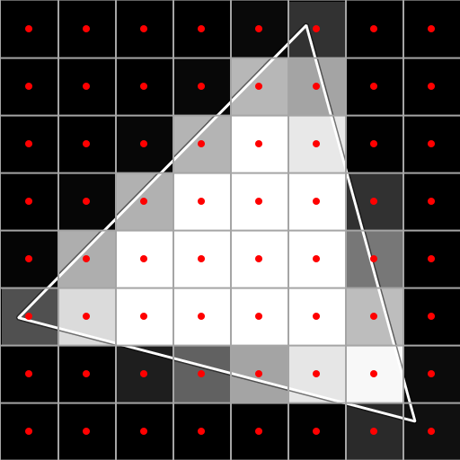
1-4. 8x8 grid with perfectly smooth output

Types of aliasing

Although all aliasing artifacts can be reduced to the problem of discretization of the representation of a continuous signal on a fixed grid consisting of a limited number of pixels, the specific reasons for their occurrence are very important for choosing an effective smoothing method that eliminates them. As will be seen later, some anti-aliasing methods can perfectly cope with the simple geometric aliasing shown in Figure 1, but fail to correct the aliasing created by other rendering processes.

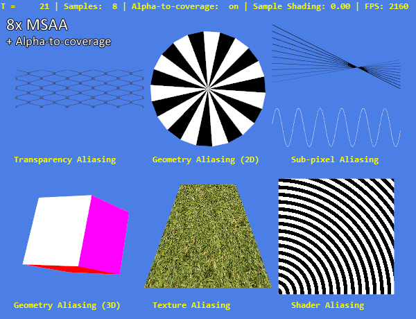
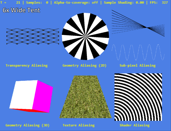
Therefore, in order to fully discuss the relative strengths and weaknesses of the anti-aliasing techniques, we grouped the aliasing artifacts arising from 3D rendering into five separate categories. This grouping depends on the exact conditions of generating artifacts. Figure 2 shows these types of aliasing with a real example, rendered using OpenGL.


Figure 2 : Different types of aliasing. From left to right, top to bottom:
• The only rectangle aligned with the screen with a partially transparent texture.
• “Mill”, consisting of alternating white and black triangles aligned with the screen.
• Several black lines of various widths, starting from 1 pixel on top to 0.4 pixels from the bottom, and a white line 0.5 in thickness, representing a sine wave.
• Cube consisting of six flat filled rectangles
• Inclined plane textured by high-frequency grass texture.
• A rectangle aligned with the screen with a pixel shader defining the color of each pixel based on the sine function.

The most common type of aliasing, which we have already mentioned, is geometric aliasing . This artifact occurs when a primitive of a scene (usually a triangle) partially overlaps with a pixel, but this partial overlap is not taken into account in the rendering process.

Transparent aliasing occurs in textured primitives with partial transparency. The top left image in Figure 2 is rendered using a single rectangle filled with a partially transparent mesh fence. Since the texture itself is just a fixed grid of pixels, it needs to be sampled at the points on which each pixel of the rendered image is superimposed, and for each such point a decision should be made whether transparency is necessary in it. As a result, the same problem of sampling arises, which we have already met on solid geometry.

Although it is actually a type of geometric aliasing, sub-pixel aliasing requires special consideration, as it sets unique problems for analytical smoothing methods that have recently gained great popularity in the rendering of games. We will look at them in detail in the article. Sub-pixel aliasing occurs when a rasterized structure is superimposed on less than one pixel in the frame buffer grid. This most often happens in the case of narrow objects - spiers, telephone or electric lines, or even swords, when they are far enough away from the camera.

Figure 3. Illustration of subpixel aliasing.


3-1. Grid 8x8 with marked centers


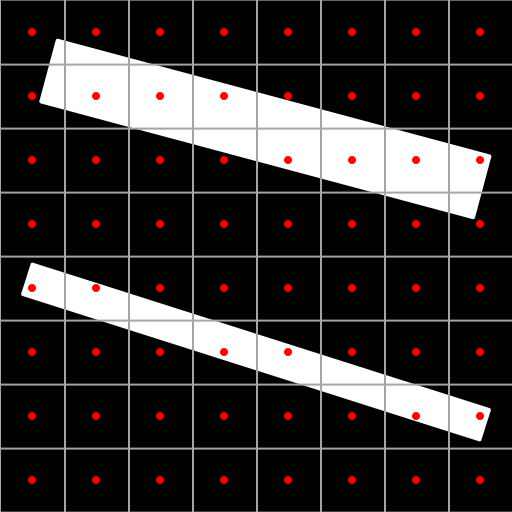
3-2. 8x8 grid with two straight line segments


3-3. Grid 8x8 with rasterized segments, without AA


3-4. 8x8 grid with perfectly smooth triangle


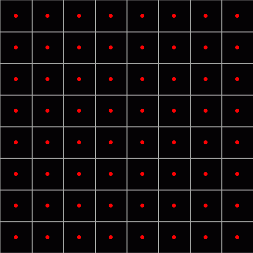
Figure 3 shows subpixel aliasing in a simple scene consisting of two straight line segments. The upper one is one pixel wide, and although during rasterization it demonstrates the familiar artifact “ladder” of geometric aliasing, the result still generally corresponds to the input data. The bottom segment is half a pixel wide. During rasterization, part of the pixel columns it intersects does not have a single pixel center within the segment. As a result, it is divided into several unrelated fragments. The same can be seen on straight lines and sinusoid curve in Figure 2.

Texture aliasing occurs when texture sampling is insufficient, especially in cases of anisotropic sampling (these are cases where the surface is strongly inclined relative to the screen). Usually, artifacts created by this type of aliasing are not obvious on fixed screenshots, but appear in motion as flickering and pixel instability. Figure 4 shows this in several frames of the sample program in animation mode.


Texture aliasing can usually be prevented by using mipmaking and filtering high-quality textures, but it still sometimes remains a problem, especially with some driver versions of popular video processors that downsamper high-anisotropic textures. It is also influenced by various anti-aliasing methods, so it is also included in the demonstration program.

And finally, shader aliasing occurs when a pixel shader program that runs for each pixel and determines its color generates a result with aliasing. This often happens in games with shaders that create contrast lighting, for example, mirror highlights based on the normal map, or with contrast lighting techniques like cel shading or back lighting. In the demonstration program, this is approximated by one shader, which calculates the sine function for the texture coordinates and paints all negative results with black, and all positive results with white.

Sampling-based smoothing techniques

Armed with an understanding of aliasing artifacts and all types of aliasing that may occur when rendering a 3D scene, we can start researching anti-aliasing techniques. These techniques can be divided into two categories: techniques trying to reduce aliasing by increasing the number of samples generated during rendering and techniques trying to mitigate the aliasing artifacts by analyzing and post-processing the generated images. The category of smoothing techniques based on sampling is simpler, so you should start with it.

Let's look again at our first example with a triangle in a 8 × 8 grid. The problem with standard rendering is that we only sample the center of each pixel, which leads to the generation of an ugly “ladder” on the edges that are not completely horizontal or vertical. On the other hand, the calculation of the coverage of each pixel is impossible in real time.

An intuitive solution would be to simply increase the number of samples taken per pixel . This concept is shown in Figure 5.


Figure 5 : A triangle rasterized with four ordered samples per pixel.

The centers of the pixels are again marked with red dots. However, in each pixel there are actually four separate places sampled (they are marked with turquoise dots). If the triangle does not close any of these samples, then the pixel is considered black, and if it covers them all, then white. Here the situation is interesting when only part of the pixels are closed: if one of the four is closed, then the pixel will be 25% white and 75% black. In the case of two of the four 50/50 ratio, and with three samples closed, the result will be a lighter shade of 75% white.

This simple idea is the foundation of all sample-based antialiasing methods. In this context, it is also worth noting that when the number of samples per pixel tends to infinity, the result of this process will tend to the “ideal” smooth example shown earlier. Obviously, the quality of the result strongly depends on the number of samples used - but also the performance. Usually in games 2 or 4 samples are used per pixel, and 8 or more are usually used only in powerful PCs.

There are other important parameters, the change of which may affect the quality of the results obtained by anti-aliasing methods based on sampling. Basically this is the location of the samples , the type of samples and the grouping of samples .

The location of the samples

The location of the samples inside the pixel greatly influences the final result, especially in the case of a small number of samples (2 or 4), which is most often used in real-time graphics. In the previous example, the samples are arranged as if they are the centers of the rendered image four times the original (16 × 16 pixels). This is intuitive and easy to achieve by simply rendering a large image size. This method is known as anti-aliasing on an ordered grid (ordered grid anti-aliasing, OGAA), also sometimes referred to as downsampling. In particular, it is implemented by a forced increase in the rendering resolution compared to the monitor resolution.

However, an ordered grid is often suboptimal, especially for almost vertical and almost horizontal lines, in which aliasing artifacts are most obvious. Figure 6 shows why this happens and how a rotated or sparse sampling grid provides much better results:


6-1. Scene with almost vertical line


6-2. Perfectly smooth rasterization


6-3. Rasterization with four ordered samples


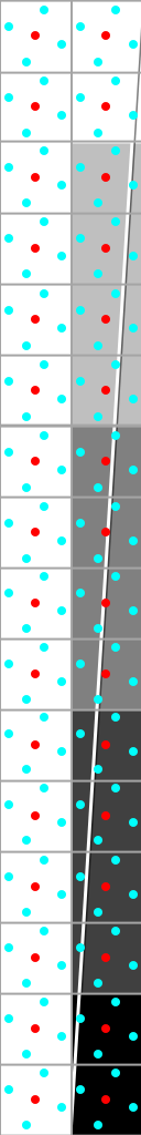
6-4. Smoothing with four sparse samples

In this almost vertical case, the ideal result with four samples should have five different shades of gray: black with completely unclosed samples, 25% white with one closed sample, 50% with two and so on. However, rasterization with an ordered grid gives us only three shades: black, white and 50/50. This happens because the ordered samples are arranged in two columns, and therefore, when one of them closes with a nearly vertical primitive, the other is also likely to be closed.

As shown in the image with a sparse sampling, this problem can be circumvented by changing the position of the samples inside each pixel. The ideal arrangement of samples for smoothing is sparse . This means that with N samples, no two samples have one common column, row or diagonal in the NxN grid. Such patterns correspond to the solutions of the N Queens problem . Antialiasing methods that use such grids are called anti-aliasing on sparse grids (sparse grid anti-aliasing, SGAA) .

Types of samples

The simplest approach to image anti-aliasing based on sampling is that all calculations are performed on the “real” pixel of each sample. Although this approach is highly efficient for removing all types of aliasing artifacts, it is also very computationally expensive, because with N samples it increases the cost of shading, rasterization, bandwidth and memory by N times. Techniques in which all calculations are performed for each individual sample are called super-sampling anti-aliasing (SSAA) .

Around the beginning of this century, support for antialiasing by multisampling (MSAA) , which is an optimization of supersampling, was built into the graphics hardware. Unlike the SSAA case, in MSAA, each pixel is shaded only once. However, for each sample, the depth and stencil values ​​are calculated, which ensures the same smoothing quality on the geometry edges as in SSAA, with a much smaller decrease in performance. In addition, further performance improvements are possible, especially for busy bandwidth, if Z-buffer and color buffer compression is supported. They are supported in all modern video processor architectures. Because of the way MSAA optimizes sampling, with aliasing transparency, textures and shaders this way cannot be done directly.

The third type of sampling was introduced by NVIDIA in 2006 in anti-aliasing technology coverage (sampling anti-aliasing, CSAA) . MSAA separates shading from pixel-by-pixel depth and stencil calculations, while CSAA adds coverage samples that do not contain color, depth, or stencil values ​​— they only store the binary value of the coverage. Such binary samples are used to assist in mixing the finished MSAA samples. That is, CSAA modes add coverage samples to MSAA modes, but it does not make sense to perform coverage sampling without creating multiple MSAA samples. Modern NVIDIA hardware uses three CSAA modes: 8xCSAA (4xMSAA / 8 coverage samples), 16xCSAA (4x / 16), 16xQCSAA (8x / 16) and 32xCSAA (8x / 32). AMD has a similar implementation with 4x EQAA (2x / 4), 8xEQAA (4x / 8) and 16xEQAA (8x / 16). Additional coverage samples are usually only marginally affected by performance.

Sample grouping

The final ingredient of AA based sampling methods is how samples are grouped, that is, how the individual samples generated during rendering are collected into the final color of each pixel. As shown in Figure 7, various grouping filters are used for this purpose. The figure shows 3 × 3 pixels — the cyan dots represent the positions of the samples, and the yellow hue indicates the sample grouping filter.


7-1. Filter Box


7-2. Quincunx Filter


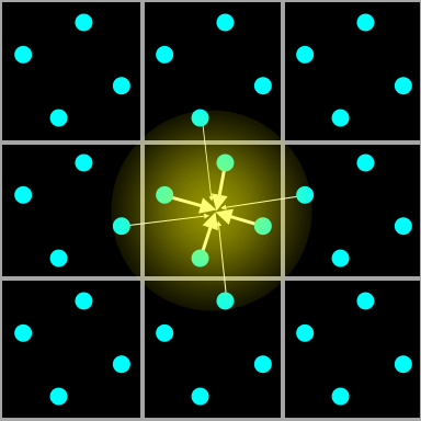
7-3. Filter tent

The obvious and most common grouping method simply accumulates each sample in a square region representing a pixel with equal weights. This is called the “box” filter, and is used in all normal MSAA modes.

One of the first approaches attempting to improve the smoothing effect with a small number of samples is anti-aliasing “quincunx”. In it, only two samples are calculated per pixel: one in the center, and one shifted up and left by half a pixel. However, instead of these two samples, the five samples that make up the pattern shown in Figure 7 accumulate. This leads to a significant reduction in aliasing, but at the same time blurs the entire image, because the color values ​​of the surrounding pixels are grouped into each pixel.

A more flexible approach was introduced in 2007 by AMD in the HD 2900 series of video processors. They use programmable grouping of samples, which allows for the implementation of the “narrow tent” and “wide tent” grouping modes. As shown above, each sample does not have the same weight. Instead, the weighting function is used, depending on the distance to the center of the pixel. Narrow (narrow) and wide (wide) options use a different size of the filter core. These grouping methods can be combined with different number of samples, and some of the results obtained are shown in a general comparison. As for quincunx AA, these methods represent a trade-off between image sharpness and aliasing reduction.

AA Sampling Comparison

Figure 8 shows a comparison of all the AA methods we considered based on sampling with a different number of samples. The image of "ground truth" shows the closest to the "real", the perfect representation of the scene. It is created by combining 8xSGSSAA and 4 × 4 OGSSAA.

It is worth noting the similar quality of SGMSAA and SGSSAA with the same number of samples with geometric aliasing, and the lack of anti-aliasing of transparency, textures and shaders in the case of MSAA. Disadvantages of ordered sampling patterns, especially for almost horizontal and almost vertical lines, are immediately noticeable when comparing 4x SGSSAA and 2 × 2 OGSSAA. With only two samples per pixel, OGSSAA is limited only to the horizontal (2 × 1) or only vertical (1 × 2) AA, and the sparse pattern to some extent can cover both types of edges.

AA methods with sample grouping filters, which are different from the usual box filter, usually provide a better reduction in aliasing per sample, but suffer from the blur effect of the entire image.

It is necessary to note one more important point - especially in the light of the subsequent discussion of AA analytical methods - all these methods based on sampling apply equally well to sub-pixel aliasing and ordinary geometric aliasing.

Figure 8 : Handling of various types of aliasing using different AA methods based on sampling.


"True" image


Without AA


2x MSAA


2x SGSSAA


4x MSAA


4x SGSSAA


8x MSAA


8x SGSSAA


8x MSAA + alpha-to-coverage


2x1 OGSSAA


1x2 OGSSAA


2x2 OGSSAA


4x Narrow Tent


6x Narrow Tent


6x Wide Tent


8x Wide Tent

Analytical antialiasing techniques

Sampling-based techniques are intuitive and work quite well with a fairly large number of samples, but at the same time they are expensive in terms of computation. This problem is exacerbated when rendering methods are used (for example, deferred shading), which can complicate the use of effective types of hardware accelerated sampling. Therefore, other ways to reduce the visual artifacts created by aliasing during 3D rendering are being explored. Such methods render a regular image with one sample per pixel, and then try to identify and eliminate aliasing by analyzing the image .

Brief introduction and introduction

Although the idea of ​​smoothing computer-generated images has been popularized thanks to Reshetov's article on morphological anti-aliasing of 2009 (often called MLAA ) [1], it is by no means new. Jules Blumenthal gave a concise description of this technique in his 1983 article for SIGGRAPH "Edge Inference with Applications to Antialiasing", which is actively used in modern methods [2]:

“The edge, sampled by points for display on the raster device, and not parallel to the display axis, looks like a ladder. , . , , , , . .

, , . , ».

In 1999, Ishiki and Kunieda presented the first version of this technique, intended for use in real time, which was performed by scanning pairs of rows and columns of an image, and could be implemented in hardware [3].

In general, all purely analytical antialiasing methods are performed in three stages:

1. Recognition of gaps in the image.
2. Recreation of geometric edges from the pattern of gaps.
3. Smoothing pixels crossing these edges by blending the colors of each side.

Separate implementations of analytical anti-aliasing differ in how these steps are implemented.

Gap Recognition

The simplest and most common way to recognize gaps is to simply study the final rendered color buffer. If the color difference between two neighboring pixels (their distance ) is greater than a certain threshold value, then there is a gap, otherwise it is not. These distance measures are often calculated in a color space that simulates human vision better than RGB, for example, in HSL .

Figure 9 shows an example of a rendered image, as well as horizontal and vertical gaps calculated from them.


Figure 9: Recognizing breaks in a color buffer. Left: image without AA. In the center: horizontal gaps. Right: vertical breaks.

To speed up the process of recognizing gaps or reduce the number of false-positive recognitions (for example, in a texture, or around the text in Figure 9), you can use other buffers generated during the rendering process. Usually, a Z-buffer (depth buffer) is available for the forward and reverse renderer. It stores the depth value for each pixel, and can be used to recognize edges. However, it only works to recognizeedge silhouettes., that is, the outer edges of the 3D object. To view the edges inside the object, you need to use another buffer instead of or in addition to the Z-buffer. For deferred renderers, a buffer is often generated that stores the direction of the normals surfaces of each pixel. In this case, the angle between adjacent normals will be a suitable metric for edge recognition.

Edge Recreation and Blending

The method of reconstructing geometric edges from discontinuities varies slightly in different analytical AA methods, but they all perform similar actions by comparing patterns on horizontal and vertical discontinuities to recognize the typical “ladder” pattern of aliasing artifacts. Figure 10 shows the patterns used according to Reshetov’s description in MLAA and the method for recreating edges.

Figure 10: MLAA patterns and their recreated edges


Recognized patterns


The discontinuity patterns used in MLAA.

After reconstructing the geometric edges, it is simple to calculate how much the top / bottom or right / left pixel along the edge should contribute to the mixed color of the pixel in order to generate a smooth appearance.

Advantages and disadvantages of analytical smoothing

Compared to sample-based antialiasing methods, analytical solutions have several important advantages. With proper operation (on properly recognized geometric edges), they can provide quality equal to the quality of sampling methods with a very high number of samples, while spending less computational resources. Moreover, they are easily applicable in many cases in which AA based on sampling is more difficult to implement, for example, in the case of deferred shading.

However, analytical AA is not a panacea. An integral problem of purely analytical methods based on a single sample is that they cannot cope with sub-pixel aliasing .

If you transfer the pixel structure shown in the upper right corner of Figure 2 to the analytical smoothing algorithm, it will not be able to understand that the separated groups of pixels actually make up the line. At this stage, there are two equally unpleasant ways to solve this problem: either blurring the pixels, reducing visible aliasing, but also destroying the details, or conservative processing of only well-defined “ladder” artifacts that are definitely caused by aliasing; however, subpixel aliasing will be preserved and distorted.

Another problem with analytical methods is false positives.. When part of an image is recognized as an edge with aliasing, but in fact it is not, it will be distorted by mixing. This is especially obvious on the text, and also requires compromises: more conservative edge recognition will lead to fewer false positives, but it will also miss some edges that actually have aliasing. On the other hand, when the edge recognition threshold is expanded, these edges will also be included, but this will lead to false positives. Since anatilistic antialiasing basically tries to extrapolate more information from a rasterized image than it actually is, it is impossible to get rid of these problems completely.

Finally, the interpretation of the edges by these methods can vary greatly depending on the difference in a single pixel. Therefore, when using single-pixel analytical anti-aliasing methods, the flickering and temporal instability of the image may increase or even be added : a single changed pixel in the original image may turn into smooth output data into a whole flickering line.

Figure 11 shows some of the successful and unsuccessful results of using AA analytical methods using the example of standard algorithms FXAA and SMAA1x. The latter is usually considered the best purely analytical single-pixel algorithm that can be used in real time.

Figure 11: AA analytical methods


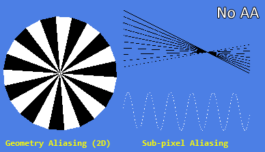
Without AA


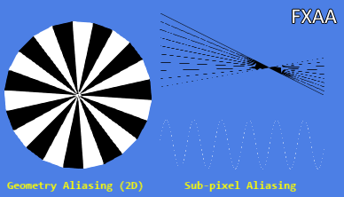
FXAA


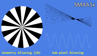
1x SMAA

Comparison of analytical antialiasing methods

Figure 12 shows a comparison between the results of FXAA, SMAA1x and the “perfect” image, and non-AA images, with 4xMSAA and 4xSGSAAA from the previous comparison.

Figure 12: Processing of various types of aliasing using different AA analytical and sampling methods


"Perfect" image


Without AA


4x MSAA


4x SGSSAA


FXAA


SMAA


Note that unlike MSAA, these analytical methods are not interested in whether geometry, transparency, or even shader calculation were the causes of aliasing artifacts. All edges are processed equally. Unfortunately, the same applies to the edges of the screen text, although the distortion with SMAA1x and less than with FXAA.

Both methods do not cope with anti-aliasing in the case of sub-pixel aliasing, however, they handle this failure differently: SMAA1x simply decides not to affect individual white pixels of the sinusoid at all, and FXAA mixes them with their surroundings. More desirable processing depends on context and personal preference.

More objectively, SMAA1x processes some angles of lines in the 2D geometry test and curves in the shader aliasing example is definitely better than FXAA, providing a smoother result that is more aesthetically pleasing and closer to the “perfect” image. This happened due to a more complicated stage of rib reconstruction and mixing, the details of which are explained in the 2012 SMAA article by Jimenez et alia [4].

Future antialiasing

We got a good understanding of the many anti-aliasing methods (analytical and based on sampling), which are now actively used in games. It is time to speculate a little. What anti-aliasing techniques can be seen on a new generation of consoles raising the bar for technology? How can the weaknesses of the existing methods be mitigated, and how will the new equipment be allowed to use new algorithms?

Well, the future is already partly here: combined methods based on sampling and analytical anti-aliasing. These algorithms create several scene samples — by means of traditional multi- or supersampling, or by temporal accumulation between frames — and combine them with analysis, generating the final image with anti-aliasing. This allows them to reduce the problems of sub-pixel aliasing and temporal instability of single-sample purely analytical methods, but still gives much better results on geometric edges than pure sampling methods with similar performance characteristics. A very simple combination of additional sampling and analytical AA can be obtained by combining single-sample analytical techniques like FXAA with subsampling from a higher resolution buffer. More sophisticated examples of such methods are SMAA T2x, SMAA S2x and SMAA 4x, as well as TXAA.The SMAA methods are explained in detail and compared inthis article , while NVIDIA implemented its own approach to TXAA here . It is highly probable that such combined methods will be more widely used in the future.

Another option, which has not yet received wide distribution, but which has great potential for the future, is to encode additional geometric information in the rendering process, which will later be used at the stage of analytical anti-aliasing. Examples of this approach are anti-aliasing with geometric post-processing (Geometric Post-process Anti-Aliasing, GPAA) and anti-aliasing using Geometry Buffer Anti-Aliasing (GBAA), the demo of which is posted here .

Finally, a common pool of CPU and video processor memory of new console platforms and future PC architectures may allow the use of technology designed to exploit such shared resources. In a recent article, “Asynchronous Adaptive Anti-aliasing Using Shared Memory,” Barringer and Moeller describe a technique that performs traditional single-sample rendering, while recognizing important pixels (for example, on the edge) and rasterizing additional sparse samples for them in the CPU [5] . Although this requires a serious restructuring of the rendering process, the results look promising.

Reference materials

[1] A. Reshetov, “Morphological antialiasing,” in Proceedings of the Conference on High Performance Graphics 2009 HPG '09 , New York, NY, USA, 2009, pp. 109–116.

[2] J. Bloomenthal, 'Edge Inference with Applications to Antialiasing', ACM SIGGRAPH Comput. Graph., Vol. 17, no. 3, pp. 157-162, Jul. 1983.

[3] T. Isshiki and H. Kunieda, 'Efficient anti-aliasing algorithm for computer generated images', in Proceedings of the 1999 IEEE International Symposium on Circuits and Systems ISCAS '99 , Orlando, FL, 1999, vol. 4, pp. 532–535.

[4] J. Jimenez, JI Echevarria, T. Sousa, and D. Gutierrez, 'SMAA: Enhanced Subpixel Morphological Antialiasing', Comput. Graph. Forum , vol. 31, no. 2pt1, pp. 355–364, May 2012.

[5] R. Barringer and T. Akenine-Möller, 'A ⁴ : asynchronous adaptive anti-aliasing using shared memory', ACM Trans. Graph. vol. 32, no. 4, pp. 100: 1–100: 10, Jul. 2013