Introduction to reinforcement training: from a multi-armed gangster to a full-fledged RL agent
Hi, Habr! Reinforcement training is one of the most promising areas of machine learning. With its help, artificial intelligence today is able to solve a wide range of tasks: from robotics and video games to modeling the behavior of customers and healthcare. In this introductory article we will explore the main idea of reinforcement learning and build our own self-learning bot from scratch.
The main difference between learning with reinforcement (reinforcement learning) and classical machine learning is that artificial intelligence is trained in the process of interaction with the environment, and not on historical data. Combining the ability of neural networks to restore complex interconnections and self-learning agent (system) in reinforcement learning, the machines achieved tremendous success, having won first in several Atari video games , and then the world go champion.
If you are accustomed to working with the tasks of teaching with a teacher, then in case of reinforcement learning there is a slightly different logic. Instead of creating an algorithm that learns to recruit “factor-correct answer” pairs, in reinforcement training, you must teach the agent to interact with the environment, independently generating these pairs. Then he will be trained on them through the system of observations (observations), wins (reward) and actions (actions).
')
It is obvious that now at each moment in time we do not have a constant correct answer, so the task becomes a bit more cunning. In this series of articles, we will create and train reinforcement training agents. Let's start with the simplest version of the agent, so that the basic idea of reinforcement learning is extremely clear, and then we move on to more complex tasks.
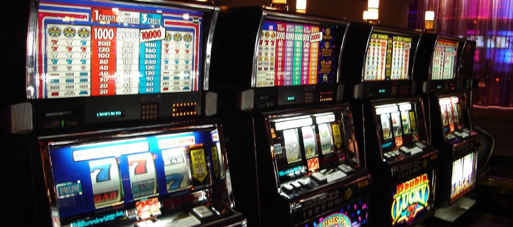
The simplest example of the task of training with reinforcements is the problem of a multi-armed gangster (it is widely covered in Habré, in particular, here and here ). In our formulation of the problem there are n slot machines, in each of which the probability of winning is fixed. Then the agent's goal is to find the slot machine with the highest expected winnings and always choose it. For simplicity, we will have only four slot machines from which to choose.
In truth, this task can with a stretch be attributed to reinforcement learning, since the following properties are characteristic of tasks from this class:
In the problem of a multi-armed gang there is neither the second nor the third condition, which simplifies it significantly and allows us to concentrate only on identifying the optimal action from all possible options. In the language of reinforcement learning, this means finding a “rule of conduct” (policy). We will use a method called policy gradients, in which the neural network updates its behavior rule as follows: the agent performs an action, receives feedback from the environment and on its basis adjusts the weights of the model through a gradient descent.
In the field of training with reinforcements, there is another approach, in which agents teach value functions. Instead of finding the optimal action in the current state, the agent learns to predict how profitable it is to be in this state and perform this action. Both approaches give good results, but the logic of the policy gradient is more obvious.
As we have already found out, in our case the expected gain of each of the gaming machines does not depend on the current state of the environment. It turns out that our neural network will consist only of a set of scales, each of which corresponds to a single gaming machine. These weights will determine which handle you need to pull to get the maximum gain. For example, if all weights are initialized to 1, then the agent will be equally optimistic about winning in all slot machines.
To update the weights of the model, we will use the e-greedy line of conduct. This means that in most cases the agent will choose an action that maximizes the expected gain, but sometimes (with a probability equal to e ) the action will be random. This will ensure that all possible options are selected, which will allow the neural network to “learn” more about each of them.
Having performed one of the actions, the agent receives feedback from the system: 1 or -1, depending on whether he won. This value is then used to calculate the loss function:
A (advantage) is an important element of all learning algorithms with reinforcement. It shows how perfect the action is better than a certain baseline. In the future, we will use a more complex baseline, but for now we take it to be 0, that is, A will simply be equal to the reward for each action (1 or -1). n is the rule of behavior, the weight of the neural network corresponding to the handle of the slot machine, which we have chosen at the current step.
It is intuitively clear that the loss function should take such values that the weights of the actions that led to the gain increase, and those that lead to the loss decrease. As a result, the weights will be updated, and the agent will increasingly choose the gaming machine with the highest fixed probability of winning, until finally he will always choose it.
Bandits First, we will create our gangsters (in everyday life the slot machine is called a gangster). In our example, they will be 4. The pullBandit function generates a random number from the standard normal distribution, and then compares it with the value of the gangster and returns the result of the game. The farther on the list is the gangster, the greater the likelihood that the agent will win by choosing him. Thus, we want our agent to learn to always choose the last gangster.
Agent. The piece of code below creates our simple agent, which consists of a set of values for thugs. Each value corresponds to a win / loss depending on the choice of a gangster. To update agent weights, we use a policy gradient, that is, we choose actions that minimize the loss function:
Agent training. We will train the agent, by choosing certain actions and receiving winnings / losses. Using the obtained values, we will know exactly how to update the weights of the model in order to more often choose gangsters with a large expected gain:
Result:
Full Jupyter Notebook can be downloaded here .
Now, when we know how to create an agent capable of choosing the optimal solution from several possible ones, let's move on to a more complex task, which will be an example of full-fledged reinforcement learning: evaluating the current state of the system, the agent must choose actions that maximize the gain not only now but in the future.
Systems in which reinforcement learning can be solved are called Markov Decision Processes (Markov Decision Processes, MDP). Such systems are characterized by winnings and actions that ensure the transition from one state to another, and these winnings depend on the current state of the system and the decision that the agent takes in this state. Winnings can be obtained with a delay in time.
Formally, the Markov decision-making process can be defined as follows. The MDP consists of a set of all possible states S and actions A , and at each moment of time it is in the state s and performs the action a of these sets. Thus, a tuple is given (s, a) and for it T (s, a) is defined - the probability of transition to the new state s' and R (s, a) is the gain. As a result, at any time in the MDP, the agent is in the state s , decides a and receives the new state s' and the gain r in response.
For example, even the process of opening the door can be represented as a Markov decision-making process. The state will be our view of the door, as well as the location of our body and the door in the world. All possible body movements that we can do are set A , and winning is the successful opening of the door. Certain actions (for example, a step in the direction of the door) bring us closer to achieving the goal, but they themselves do not bring any gain, since it is provided only by directly opening the door. As a result, the agent must perform such actions, which sooner or later lead to the solution of the problem.
Let's use OpenAI Gym - a platform for developing and training AI bots using games and algorithmic tests and take the classic task from there: the task of stabilizing an inverted pendulum or Cart-Pole. In our case, the essence of the task is to keep the rod in a vertical position as long as possible, moving the cart horizontally:
Unlike the multi-armed gangster problem, this system has:
To take into account the time lag, we need to use the policy gradient method with some corrections. First, it is now necessary to update an agent that has more than one observation per unit of time. To do this, we will collect all the observations in the buffer, and then use them simultaneously to update the model weights. This set of observations per unit of time is then compared with the discounted gain.
Thus, every action of the agent will be made taking into account not only the instant win, but all subsequent ones. Also now we will use the adjusted gain as an estimate of the A (advantage) element in the loss function.
Import the libraries and load the Cart-Pole task environment:
Agent. First, create a function that will discount all subsequent wins to the current moment:
Now create our agent:
Agent training. Now, finally, let's get to the agent's training:
Result:
You can see the complete Jupyter Notebook here . See you in the next articles, where we will continue to study reinforced learning!
Introduction
The main difference between learning with reinforcement (reinforcement learning) and classical machine learning is that artificial intelligence is trained in the process of interaction with the environment, and not on historical data. Combining the ability of neural networks to restore complex interconnections and self-learning agent (system) in reinforcement learning, the machines achieved tremendous success, having won first in several Atari video games , and then the world go champion.
If you are accustomed to working with the tasks of teaching with a teacher, then in case of reinforcement learning there is a slightly different logic. Instead of creating an algorithm that learns to recruit “factor-correct answer” pairs, in reinforcement training, you must teach the agent to interact with the environment, independently generating these pairs. Then he will be trained on them through the system of observations (observations), wins (reward) and actions (actions).
')
It is obvious that now at each moment in time we do not have a constant correct answer, so the task becomes a bit more cunning. In this series of articles, we will create and train reinforcement training agents. Let's start with the simplest version of the agent, so that the basic idea of reinforcement learning is extremely clear, and then we move on to more complex tasks.
Multi-armed bandit
The simplest example of the task of training with reinforcements is the problem of a multi-armed gangster (it is widely covered in Habré, in particular, here and here ). In our formulation of the problem there are n slot machines, in each of which the probability of winning is fixed. Then the agent's goal is to find the slot machine with the highest expected winnings and always choose it. For simplicity, we will have only four slot machines from which to choose.
In truth, this task can with a stretch be attributed to reinforcement learning, since the following properties are characteristic of tasks from this class:
- Different actions lead to different wins. For example, when searching for treasures in a maze, turning left may mean a bunch of diamonds, and turning right will mean a hole of poisonous snakes.
- The agent receives the gain with a delay in time. This means that, turning left in the maze, we do not immediately realize that this is the right choice.
- Winning depends on the current state of the system. Continuing the example above, turning left may be correct in the current part of the maze, but not necessarily in the rest.
In the problem of a multi-armed gang there is neither the second nor the third condition, which simplifies it significantly and allows us to concentrate only on identifying the optimal action from all possible options. In the language of reinforcement learning, this means finding a “rule of conduct” (policy). We will use a method called policy gradients, in which the neural network updates its behavior rule as follows: the agent performs an action, receives feedback from the environment and on its basis adjusts the weights of the model through a gradient descent.
In the field of training with reinforcements, there is another approach, in which agents teach value functions. Instead of finding the optimal action in the current state, the agent learns to predict how profitable it is to be in this state and perform this action. Both approaches give good results, but the logic of the policy gradient is more obvious.
Policy gradient
As we have already found out, in our case the expected gain of each of the gaming machines does not depend on the current state of the environment. It turns out that our neural network will consist only of a set of scales, each of which corresponds to a single gaming machine. These weights will determine which handle you need to pull to get the maximum gain. For example, if all weights are initialized to 1, then the agent will be equally optimistic about winning in all slot machines.
To update the weights of the model, we will use the e-greedy line of conduct. This means that in most cases the agent will choose an action that maximizes the expected gain, but sometimes (with a probability equal to e ) the action will be random. This will ensure that all possible options are selected, which will allow the neural network to “learn” more about each of them.
Having performed one of the actions, the agent receives feedback from the system: 1 or -1, depending on whether he won. This value is then used to calculate the loss function:
A (advantage) is an important element of all learning algorithms with reinforcement. It shows how perfect the action is better than a certain baseline. In the future, we will use a more complex baseline, but for now we take it to be 0, that is, A will simply be equal to the reward for each action (1 or -1). n is the rule of behavior, the weight of the neural network corresponding to the handle of the slot machine, which we have chosen at the current step.
It is intuitively clear that the loss function should take such values that the weights of the actions that led to the gain increase, and those that lead to the loss decrease. As a result, the weights will be updated, and the agent will increasingly choose the gaming machine with the highest fixed probability of winning, until finally he will always choose it.
Algorithm implementation
Bandits First, we will create our gangsters (in everyday life the slot machine is called a gangster). In our example, they will be 4. The pullBandit function generates a random number from the standard normal distribution, and then compares it with the value of the gangster and returns the result of the game. The farther on the list is the gangster, the greater the likelihood that the agent will win by choosing him. Thus, we want our agent to learn to always choose the last gangster.
import tensorflow as tf import numpy as np # . №4 . bandits = [0.2,0,-0.2,-5] num_bandits = len(bandits) def pullBandit(bandit): # result = np.random.randn(1) if result > bandit: # return 1 else: # return -1 Agent. The piece of code below creates our simple agent, which consists of a set of values for thugs. Each value corresponds to a win / loss depending on the choice of a gangster. To update agent weights, we use a policy gradient, that is, we choose actions that minimize the loss function:
tf.reset_default_graph() # 2 feed-forward . . weights = tf.Variable(tf.ones([num_bandits])) chosen_action = tf.argmax(weights,0) # 6 . , . reward_holder = tf.placeholder(shape=[1],dtype=tf.float32) action_holder = tf.placeholder(shape=[1],dtype=tf.int32) responsible_weight = tf.slice(weights,action_holder,[1]) loss = -(tf.log(responsible_weight)*reward_holder) optimizer = tf.train.GradientDescentOptimizer(learning_rate=0.001) update = optimizer.minimize(loss) Agent training. We will train the agent, by choosing certain actions and receiving winnings / losses. Using the obtained values, we will know exactly how to update the weights of the model in order to more often choose gangsters with a large expected gain:
total_episodes = 1000 # total_reward = np.zeros(num_bandits) # 0 e = 0.1 # init = tf.global_variables_initializer() # tensorflow with tf.Session() as sess: sess.run(init) i = 0 while i < total_episodes: # if np.random.rand(1) < e: action = np.random.randint(num_bandits) else: action = sess.run(chosen_action) # , reward = pullBandit(bandits[action]) # _,resp,ww = sess.run([update,responsible_weight,weights], feed_dict={reward_holder:[reward],action_holder:[action]}) # total_reward[action] += reward if i % 50 == 0: print(" " + str(num_bandits) + " bandits: " + str(total_reward)) i+=1 print(" , №" + str(np.argmax(ww)+1) + " ...") if np.argmax(ww) == np.argmax(-np.array(bandits)): print("... !") else: print("... !") Result:
4 : [-1. 0. 0. 0.] 4 : [ -1. -1. 0. 45.] 4 : [ -2. -1. 1. 91.] 4 : [ -3. -1. 1. 138.] 4 : [ -2. 0. 2. 183.] 4 : [ 0. 0. 2. 229.] 4 : [ -1. 0. 3. 277.] 4 : [ -1. -1. 4. 323.] 4 : [ -2. -1. 2. 370.] 4 : [ -2. -2. 3. 416.] 4 : [ -2. -2. 3. 464.] 4 : [ -3. -1. 3. 508.] 4 : [ -7. 1. 4. 549.] 4 : [ -9. 0. 3. 593.] 4 : [ -9. 0. 4. 640.] 4 : [ -9. 0. 5. 687.] 4 : [ -9. -2. 5. 735.] 4 : [ -9. -4. 7. 781.] 4 : [ -10. -4. 8. 829.] 4 : [ -13. -4. 7. 875.] , №4 ... ... ! Full Jupyter Notebook can be downloaded here .
The solution to the full-fledged learning problem with reinforcement
Now, when we know how to create an agent capable of choosing the optimal solution from several possible ones, let's move on to a more complex task, which will be an example of full-fledged reinforcement learning: evaluating the current state of the system, the agent must choose actions that maximize the gain not only now but in the future.
Systems in which reinforcement learning can be solved are called Markov Decision Processes (Markov Decision Processes, MDP). Such systems are characterized by winnings and actions that ensure the transition from one state to another, and these winnings depend on the current state of the system and the decision that the agent takes in this state. Winnings can be obtained with a delay in time.
Formally, the Markov decision-making process can be defined as follows. The MDP consists of a set of all possible states S and actions A , and at each moment of time it is in the state s and performs the action a of these sets. Thus, a tuple is given (s, a) and for it T (s, a) is defined - the probability of transition to the new state s' and R (s, a) is the gain. As a result, at any time in the MDP, the agent is in the state s , decides a and receives the new state s' and the gain r in response.
For example, even the process of opening the door can be represented as a Markov decision-making process. The state will be our view of the door, as well as the location of our body and the door in the world. All possible body movements that we can do are set A , and winning is the successful opening of the door. Certain actions (for example, a step in the direction of the door) bring us closer to achieving the goal, but they themselves do not bring any gain, since it is provided only by directly opening the door. As a result, the agent must perform such actions, which sooner or later lead to the solution of the problem.
The task of stabilizing an inverted pendulum
Let's use OpenAI Gym - a platform for developing and training AI bots using games and algorithmic tests and take the classic task from there: the task of stabilizing an inverted pendulum or Cart-Pole. In our case, the essence of the task is to keep the rod in a vertical position as long as possible, moving the cart horizontally:
Unlike the multi-armed gangster problem, this system has:
- Observations. The agent must know where the rod is now and at what angle. This observation will be used by the neural network to assess the likelihood of a particular action.
- Delayed winnings It is necessary to move the cart in such a way that it is beneficial both at the moment and in the future. To do this, we will compare the pair “observation - action” with the adjusted value of the gain. Adjustment is performed by a function that weighs actions by time.
To take into account the time lag, we need to use the policy gradient method with some corrections. First, it is now necessary to update an agent that has more than one observation per unit of time. To do this, we will collect all the observations in the buffer, and then use them simultaneously to update the model weights. This set of observations per unit of time is then compared with the discounted gain.
Thus, every action of the agent will be made taking into account not only the instant win, but all subsequent ones. Also now we will use the adjusted gain as an estimate of the A (advantage) element in the loss function.
Algorithm implementation
Import the libraries and load the Cart-Pole task environment:
import tensorflow as tf import tensorflow.contrib.slim as slim import numpy as np import gym import matplotlib.pyplot as plt %matplotlib inline try: xrange = xrange except: xrange = range env = gym.make('CartPole-v0') # Agent. First, create a function that will discount all subsequent wins to the current moment:
gamma = 0.99 # def discount_rewards(r): """ , """ discounted_r = np.zeros_like(r) running_add = 0 for t in reversed(xrange(0, r.size)): running_add = running_add * gamma + r[t] discounted_r[t] = running_add return discounted_r Now create our agent:
class agent(): def __init__(self, lr, s_size,a_size,h_size): # feed-forward . # self.state_in= tf.placeholder(shape=[None,s_size],dtype=tf.float32) hidden = slim.fully_connected(self.state_in,h_size, biases_initializer=None,activation_fn=tf.nn.relu) self.output = slim.fully_connected(hidden,a_size, activation_fn=tf.nn.softmax,biases_initializer=None) self.chosen_action = tf.argmax(self.output,1) # # 6 . # # , # . self.reward_holder = tf.placeholder(shape=[None],dtype=tf.float32) self.action_holder = tf.placeholder(shape=[None],dtype=tf.int32) self.indexes = tf.range(0, tf.shape(self.output)[0])*tf.shape(self.output)[1] + self.action_holder self.responsible_outputs = tf.gather(tf.reshape(self.output, [-1]), self.indexes) # self.loss = -tf.reduce_mean(tf.log(self.responsible_outputs)* self.reward_holder) tvars = tf.trainable_variables() self.gradient_holders = [] for idx,var in enumerate(tvars): placeholder = tf.placeholder(tf.float32,name=str(idx)+'_holder') self.gradient_holders.append(placeholder) self.gradients = tf.gradients(self.loss,tvars) optimizer = tf.train.AdamOptimizer(learning_rate=lr) self.update_batch = optimizer.apply_gradients(zip(self.gradient_holders, tvars)) Agent training. Now, finally, let's get to the agent's training:
tf.reset_default_graph() # tensorflow myAgent = agent(lr=1e-2,s_size=4,a_size=2,h_size=8) # total_episodes = 5000 # max_ep = 999 update_frequency = 5 init = tf.global_variables_initializer() # tensorflow with tf.Session() as sess: sess.run(init) i = 0 total_reward = [] total_lenght = [] gradBuffer = sess.run(tf.trainable_variables()) for ix,grad in enumerate(gradBuffer): gradBuffer[ix] = grad * 0 while i < total_episodes: s = env.reset() running_reward = 0 ep_history = [] for j in range(max_ep): # , a_dist = sess.run(myAgent.output,feed_dict={myAgent.state_in:[s]}) a = np.random.choice(a_dist[0],p=a_dist[0]) a = np.argmax(a_dist == a) s1,r,d,_ = env.step(a) # ep_history.append([s,a,r,s1]) s = s1 running_reward += r if d == True: # ep_history = np.array(ep_history) ep_history[:,2] = discount_rewards(ep_history[:,2]) feed_dict = {myAgent.reward_holder:ep_history[:,2], myAgent.action_holder:ep_history[:,1], myAgent.state_in:np.vstack(ep_history[:,0])} grads = sess.run(myAgent.gradients, feed_dict=feed_dict) for idx,grad in enumerate(grads): gradBuffer[idx] += grad if i % update_frequency == 0 and i != 0: feed_dict = dictionary = dict(zip(myAgent.gradient_holders, gradBuffer)) _ = sess.run(myAgent.update_batch, feed_dict=feed_dict) for ix,grad in enumerate(gradBuffer): gradBuffer[ix] = grad * 0 total_reward.append(running_reward) total_lenght.append(j) break # if i % 100 == 0: print(np.mean(total_reward[-100:])) i += 1 Result:
16.0 21.47 25.57 38.03 43.59 53.05 67.38 90.44 120.19 131.75 162.65 156.48 168.18 181.43 You can see the complete Jupyter Notebook here . See you in the next articles, where we will continue to study reinforced learning!
Source: https://habr.com/ru/post/343834/
All Articles