Heading "We read articles for you." October - November 2017

Hi, Habr! By tradition, we present to your attention a dozen reviews of research papers from members of the Open Data Science community from the #article_essense channel. Want to get them before everyone else - join the ODS community!

Articles are selected either from personal interest, or because of the proximity to the ongoing competition. We remind you that the descriptions of the articles are given without changes and in the form in which the authors posted them in the #article_essence channel. If you want to offer your article or you have any suggestions - just write in the comments and we will try to take everything into account in the future.

Articles for today:

1. Combining Number Of Neural Networks Into One
2. AutoEncoder by Forest
3. Name-Entity Recognition (NLP) of the Hybrid LSTM-CRF
4. Densely Connected Convolutional Networks (CV)
5. Dual Path Networks (CV)
6. A Large Self-Annotated Corpus for Sarcasm (NLP)
7. Fashion-MNIST: a Novel Image Dataset for Benchmarking Machine Learning Algorithms (CV)
8. Dynamic Routing Between Capsules (Hinton's capsules)
9. DeepXplore: Automated Whitebox Testing of Deep Learning Systems
10. One-Shot Learning for Semantic Segmentation (CV)
11. Field-aware Factorization Machines in a Real-World Online Advertising System
12. The Marginal Value of Adaptive Gradient Methods in Machine Learning
13. FractalNet: Ultra-Deep Neural Networks without Residuals (CV)

1. Combining Infinity Number Of Neural Networks Into One

Article authors: Bo Tian, ​​2016
→ Original article
Review author: BelerafonL

The idea is to add Gaussian noise to the weights of the neurons to get something like a drop-out. Only if the dropout usually acts on the outputs of the nodes, then the noise is added to the weights. But this is not the main thing, but the fact that the author finds an analytical solution for network output with an endless ensemble of such networks with a different combination of noise samples in the scales. Those. The desired noise level of the scale (sigma) is specified, and the solution found shows what the network would produce if it were to sample the output of such a noisy network for a long time and to average the result.

The author for the problem of separating two spirals on a plane shows how the solution of a conventional network differs from that. He draws an activation card, and for a normal network, and it turns out to be rugged and torn, and to solve it, it is smooth and exactly follows the shape of the spirals.
Unfortunately, the author does not check the proposed method for other tasks and uses the network with only one hidden layer. In addition, he uses the LMA optimization method (Levenberg – Marquardt Algorithm), but says that you can use any other, including the usual backprop.

The article’s premise is simple - an endless ensemble of networks differing by the amount of noise in the scales perfectly generalizes and finds the best minimum, besides, the noise level of the scales can be changed as the network is trained, and then the desired accuracy / generalization ratio can be found. And since the solution is found analytical, the computational cost of this is almost none.

There are a lot of formulas in the article, why I did not understand the applicability of the method for practical complex problems, are there any pitfalls. Therefore, I ask more experienced researchers to look at and comment on the article, it is painfully beautiful to get the result of such regularization.

Also there is an author's note on stackexchange where he briefly explains the concept.

2. AutoEncoder by Forest

Article authors: Zhou Z, Feng J, 2017
→ Original article
Reviewer : Dumbris

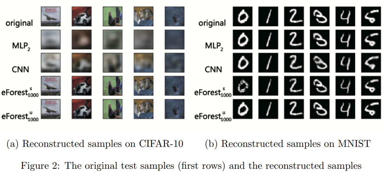
In the article AutoEncoder by Forest, the authors of Zhou Z, Feng J proposed an alternative method of building auto-encoders based on an ensemble (Random Forest, Gradient boosted tree) of trees. They called the proposed method eForest .

According to the authors' experiments, eForest shows the best results on the MNIST and CIFAR-10 tasks, in comparison with auto-encoders built on the basis of the Multilayer Perceptron and Convolutional Neural Network. And in the task of recovering text on the IMDB dataset, eForest exceeded MLP accuracy 200 times.

The main advantages of the eForest method:

• Accuracy : reconstruction error is lower than that of NN-based auto-encoders
• Efficiency : learning on a multi-core CPU is faster than NN using a GPU (but, while the decoding phase in eForest is slow)
• damage-tolerable - the model works upon partially erasing the encoded representation. In experiments with the text even for the remaining 10%, the model was able to show an acceptable result.
• reusable eForest-trained auto-encoders can be used on other data from the same domain domain.

How does the proposed method work

The autoencoder has two main functions encoding and decoding.
Coding To obtain an encoded representation, you need to construct a forest F trees T and save the indexes of sheets from all trees for each x . Thus, for input x we obtain a vector of long T.

Decoding - having a forest F and sheet indexes for all x you can restore the path in the tree from sheet to top. The authors write this way in the form of a conjunction of logical expressions taken from the nodes of the decision tree. Example (x1=>0)^(x2=>5)^:(x3==RED)^:(x1>2:7)^:(x4 == NO) . Such an expression they call RULE.

Many RULEs for a particular sample from all T trees can be simplified, to one rule, which Zhou Z, Feng J call: Maximal-Compatible Rule (MCR). The authors claim, in the form of a theorem, that all original samples will be located within the regions defined by the MCR.

According to the rules recorded in the MCR, you can generate data that will be similar to the original. The article has a description of the algorithms in pseudo-code format.

Judging from Table 4, the procedure for constructing MCR and decoding takes much longer, compared to the decoding phase in NN. But the authors hope to optimize this moment in the future.

At the beginning of the year, there was a more general paper from these same authors: Deep Forest: Towards .

3. Application of a Hybrid Bi-LSTM-CRF Named Entity Recognition

Authors of the article: Anh LT Arkhipov M. Y, Burtsev M. S, 2017
→ Original article
Reviewer : Dumbris

The first publication in the project iPavlov . According to the authors - SOTA for NER in Russian texts.

Datasets

For the experiments, Gareev's datasets (top cited articles from Yandex News), Person-1000 and FactRuEval were used. As a baseline, a Bi-LSTM network was taken with a Conditional Random Fields (CRF) layer. The use of CRF gives a significant increase in accuracy compared to pure Bi-LSTM on the NER task.

Network architecture, experiments

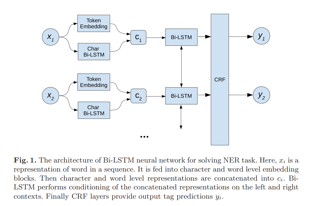
At the input for each word its word level and char level representation is calculated, both representations are concatenated into one vector and fed to the input Bi-LSTM. After Bi-LSTM, the CRF layer assigns to each word a tag by which it can be determined whether the word is a person’s name or an organization’s name.

During the experiments, extensions of the well-known NeuroNER architecture were also investigated using the highway network. With the highway network, the network gets the opportunity to learn to “turn off” some of the inner layers (carry gate), skipping low-level views of the input data closer to the output layers. This mechanism is implemented using the sigmoid layer. It turns out that the network itself can manage the complexity of the architecture, depending on the input data.

However, in practice it was found that the use of properly prepared word embeddings gives an increase in accuracy in combination with Bi-LSTM-CRF. For training embeddings, News by Kutuzov and Lenta corps were used.

results

The most accurate was the model Bi-LSTM-CRF + word embedding, created on the basis of Russian news corpses. The combination of NeuroNER + highway network also performed well. One of the promising directions is the use of character level CNN architecture, instead of LSTM. In the framework of this work it has not been investigated.

4. Densely Connected Convolutional Networks

Authors: Gao Huang, Zhuang Liu, Kilian Q. Weinberger, Laurens van der Maaten, 2016
→ Original article
Reviewed by : N01Z3

A relatively fresh idea of ​​the architecture, which passed somehow unnoticed, but showed in our Chata the best single model performance on Kaggle Amazon from Space .

So the guys offered the Dense Block. Each base element is BN -> ReLU -> Conv. And each basic element prokidyvaet its features to all the following elements in the block. Features are concatenated, not aggregated, so the number of channels grows linearly in the number of filters (the authors call this Growth rate). But this is offset by the fact that the basic elements themselves are narrower. Also, in order to reduce the increase in the number of channels after each Dense Block, a basic element is inserted with convolutions (1, 1) and the number of filters is two times less than the channels at this point in the main branch. And then the usual Pooling with Stride 2.

Everything. And then waving hands goes on, that the features are more competently re-used, that due to this, everything is effectively considered. Even in this case, the dropout in convolutions looks somehow more meaningful. Also in the following papers, the guys showed that it is possible to get an evaluation classification already after the first blocks and thus not to drive the inference further in the case of confident predictions.

5. Dual Path Networks

Authors of the article: Yunpeng Chen, Jianan Li, Huaxin Xiao, Xiaojie Jin, Shuicheng Yan, Jiashi Feng, 2017
→ Original Article → Source Code
Reviewed by : N01Z3

Another rethinking of the connection between convolutional and recurrent networks. For starters, the authors liked Resnet and Densnet. The first is the essence of the recurrent network deployed along the main brunch, and the second is the high order recurrent sit (HORNN) (a series of pictures 1). And the guys decided to merge both ideas into one. This is how DPN was born.

To understand how they combined, a series of pictures 2

a) Classic Resnet - fixed-size main brunch, features added
b) normal Densenet - the main brunch grows, features are konkatiniruyutsya
c) conventional Densenet - equivalent circuit. Rethinking in the sense that after all there is a fixed-size basic brunch from the entrance to the DenseBlock and the auxiliary one that is growing.
d) the latest Dual Path block - there is a fixed-size brunch, there is a brunch that is growing. Features are taken from each, run through a layer of convolutions, are separated and docked in each brunch. In the fixed brunch - folded, in the growing - concatenated
e) the latest Dual Path block - equivalent Dual Path circuit.

Each input and output block uses convolutions (1.1) to match the channels. And the main convolutions (3.3) are used not ordinary, but Separable. That is, in fact, not Resnet, but ResNeXt is taken as the base.

6. A Large Self-Annotated Corpus for Sarcasm

Authors of the article: Mikhail Khodak, Nikunj Saunshi, Kiran Vodrahalli, 2017
→ Original article
Reviewed by : yorko

Recognizing sarcasm is a very non-trivial task, which is not something that grids, and people do not always cope. If a person with his 10 ^ 10 neurons sometimes asks, “Wait a minute ... and you don’t troll me by chance?”, Then you can imagine that recognizing sarcasm is really one of the greatest machine learning challenges.

Dudes have marked the biggest currently dataset on sarcasm - 1.3 million sarcastic statements with Reddit. In addition, there are still half a billion non-sarcastic phrases lying around, so that you can practice imbalanced classification at your leisure.

The guys immediately stated that their main contribution is dataset, and not the methodology for identifying sarcasm. But dataset an order of magnitude more previous and much better, according to them, than from Twitter, where people put the tags #sarcasm or #irony themselves. On Reddite, users also notice that they are tagged with the “/ s” tag, and the authors acknowledge that this markup is also noisy.

It is curious that the dudes did not collect messages going to the thread after sarcastic approval. Type there goes a trash-trolling, sarcasm respond to sarcasm, and the markup is too noisy turns out.

The authors assessed the quality of the resulting markup by selecting 500 random sarcastic and ordinary messages and checking the markup on their own. They fixed 1% False Positive Rate (when the regular message came with the label “sarcasm”) and 2% False Negative. In the case of balanced learning, these are norms, but if you study with a bunch of non-sarcasm (99.75%), then 2% False Negative Rate is a bit too much.

I'd add: I figured the error matrix for the markup with Reddit and the assessor markup, with such an imbalance the accuracy (precision) of the markup with Reddit is very low: only 11% of cases assessors confirm sarcasm, if Reddit has come to be sarcasm. This raises questions: why is it so much better than the rest, of the same Twitter? The authors argue that it’s still better: reddit comes up with sarcasm much more often (~ 1% vs. 0.002% on Twitter) and generally the message on Reddite is obviously longer. Well, ok ... persuaded

Further, the authors report several baselines in the task of determining sarcasm on Reddit's data. The task is formulated as follows: there is a message to read and all comments to it. It is necessary to determine which of the comments carry sarcasm. 8.4 million such messages were collected (as I understood, the object is the original message + comments to it), sarcasm - 28% (balanced the sample). Then they took one message from the thread with or without sarcasm, and on the basis of GloVe-embeddings, sarcastic phrases too similar to each other (avalanche-like yeast throwing shit) were cut off.

Three logistic regressions were built, the signs are very simple: Bag of Words, Bag of bigrams and GloVe-embeddings (Amazon product corpus, dimension - 1600, document presentation (messages) - simple averaging of individual words). They also planted poor assessors to mark sarcasm - there were 5 people, they marked out 100 messages, it would be a little bit difficult, it would be possible to strain a mechanical Turk (Amazon Mechanical Turk), because writing a scientific article is such a profitable business!

It turned out that the bigrams gave the best result among the three models (~ 76% accuracy in politics and 71% in the other subreddits), but the human marking is certainly better (83% and 82% on average, 85% and 92% ensemble 5 assessors, majority voting). The authors conclude that embeddingdings played worse, but it is possible, with their help, we will learn to convey the context in which sarcasm is applied.

In general, it is difficult for both people and algorithms to detect sarcasm. I expect progress in this task on the part of neural networks - we must somehow learn to properly take into account the context in which sarcasm is used, that is, correctly encode this context into a hidden representation, as it is now done in conditioned recurrent meshes. The experiments in this article are so-so, but the fact that the guys posted a big dataset of sarcasm is definitely great! I'm afraid to imagine what will happen when cars really learn to feel sarcasm better than people.

7. Fashion-MNIST: a Novel Image for Benchmarking Machine Learning Algorithms

Authors of the article: Han Xiao, Kashif Rasul, Roland Vollgraf, 2017
→ Original article
Review author: Ivan Bendyna

The guys from Zalando also burn from the phrase "state-of-the-art on MNIST", so they made their Fashion-mnist, which completely repeats the structure of the original MNIST. It also has 10 classes (clothes and shoes: shirt, t-shirt, sneakers, ...), 28x28 pixels, 60,000 train, 10,000 test. This is the main idea of ​​dataset - you can simply replace the URL and check the quality on a slightly more complex dataset. SOTA top-1 error is about 3.5%, which is an order of magnitude larger than the error on MNIST.

There is a benchmark of the main classifiers from sklearn , top results can be found in Readme.md . Also there you can find the result of a person who is only 0.835, which is not surprising in principle if you look at the pictures with your eyes.

Dataset prepared for products from the site zalando, the procedure for creating dataset well described in the work. Dataset is already in pytorch .

I also learned from the article that there is an extended dataset EMNIST (62 classes of handwritten characters)

My thoughts:

• Pictures are made from photos of clothes, that is closer in 2d-structure to ordinary photos than handwritten text
• The main drawback of MNIST has not gone away - good methods may not show improvements on such small pictures.
• Probably, this dataset will not be able to reach accuracy 0.99, since the border between some classes (for example, shirt and t-shirt) is rather arbitrary, and if it exists, it can disappear with decreasing size and translation into b / w image
• It’s not a fact that it can be a replacement, but now all those who evaluated quality on MNIST can check it for fashion mnist for free (in terms of developer time)
• Also a good alternative for homework for students who usually do not have the capacity to run on ImageNet

8. Dynamic Routing Between Capsules

Authors: Sara Sabour, Nicholas Frosst, Geoffrey E Hinton , 2017
→ Original article
Reviewer: Ruslan Grimov

This article reveals the internal structure of the capsules and describes the routing mechanism - a way to transfer the output from the capsule in the current layer only to certain capsules in the upper layer. They call this the construction of the Parse tree, where each node is associated with one capsule.

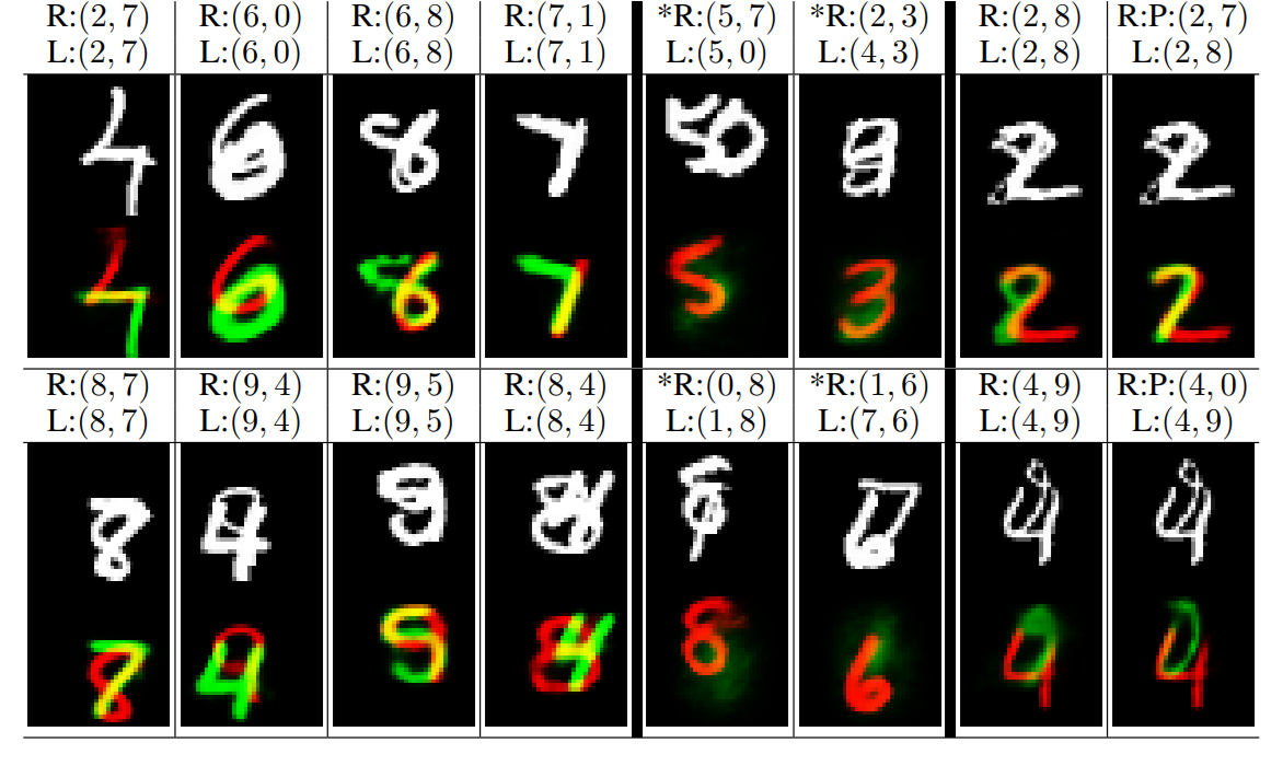
Result of the article: building an encoder / decoder trained in MNIST and calling for studying the capsules further. Encoder - CapsNet network, consists of a usual convolutional layer and two layers with capsules, one of which is convolutional (see below). A decoder is just a fullconnected network. The code supplied to the decoder is 10 capsules with 16 neurons each. One by one.

The capsule is a separate group of neurons on the layer. They are not connected to each other inside the capsule, but the output of each neuron depends on the output of the others in the capsule (see formulas below). A separate capsule is responsible for one object. Each neuron in the capsule learns to represent some property of the object. At the end of the article there will be a picture where they show how the shape of numbers changes as the properties change (it looks like these neurons really know something).

Neurons are in the same position, but in different capsules of one layer they are responsible for different properties of objects (as far as I understood). The very presence of an object on the scene is determined by the length of the output vector of the capsule (the root of the sum of the squares of neuron activities in the capsule). Respectively. if there are two identical objects on the stage, then the properties will be mixed.

The dimension of the capsules grows from the input layer of the network to the output. At the same time, information from the “positional” is transformed into a rate-coded (“rate-coded”). Simple convolutional layers at the beginning of the network are considered as capsules having one neuron.

Capsules

In the article, everything is repelled by capsules. Therefore, further all actions are described in relation to capsules, and not to individual neurons. That is, not input / output of the neuron and weights between the neurons, but input / output and weights between the capsules are considered. We simply mean that a capsule is a vector of neurons.

Routing

The length of the output vector of the capsule is less than 1. And once the length of the output vector of the capsules is normalized, it is possible to find out which of the capsules of the overlying layer are more “responsive” and transfer data from the underlying capsule only to those capsules for which the inner product U [i, j] and v [j] more. Actually this is the construction of the parsing tree (as I understood it).

The parsing tree between the l and (l + 1) layers is built on the fly (again when submitting each image).
To build this tree, special weights b [i, j] (scalar) between the capsules of the two layers are used (they are used in calculating that c [i, j] - coefficient of connectivity, but they are not permanently stored, when the new input to the network is reset to zero).

c [i, j] are calculated as exp (b [i, j]) / (sum over k from exp (b [i, k])), where k is the number of groups in the overlying layer. Those. this is softmax.

 1: procedure ROUTING(U[i,j], r, l) //prediction (  ?), - ,   2:         for all capsule i in layer l and capsule j in layer (l + 1): b[i,j] = 0 3:         for r iterations do 4:                    for all capsule i in layer l and capsule j in layer (l + 1):  c[i, j] 5:                    for all capsule j in layer (l + 1):  s[j] 6:                    for all capsule j in layer (l + 1):  v[j] 7:                    for all capsule i in layer l and capsule j in layer (l + 1): b[i,j] = b[i,j] + U[i, j]*v[j] 8:         return v[j] 

Error function

Maximize the length of the output vector of the capsule, which should be activated on the current image and minimize those that should not. Namely, we calculate the sum over all k from 0 to 9

L [k] = T max (0, 0.9 - || v [k] ||) ^ 2 + 0.5 (1 - T) * max (0, || v [k] || - 0.1) ^ 2
where T = 1 in the presence of the digit k in the picture and is equal to 0 in the absence.

In addition, we add a pixel-by-pixel error of the picture recovery by the decoder (see below), but they are added with a very small coefficient of 0.0005.

CapsNet architecture

The encoder consists of:

1. A normal convolutional layer with 256 cores 9x9, step 1 and ReLU as an activation function.
2. Layer "primary capsule", a layer with capsules, convolutional. 32 cores 9x9 of 8D capsules (8 neurons in the capsule) and in step 2. Each such capsule sees 81x256 neurons from the previous layer. In total, the second layer has [32, 6, 6] capsule exits, each of which consists of 8 neurons. Each capsule in the grid [6, 6] shares its weights with the others (it’s not quite clear how c [i, j] is calculated here, what is k? 32 or 32x6x6?).
3. Layer "DigitCaps" consists of 10 capsules 16D, each capsule is connected to all capsules of the previous layer.

Routing is used only between the second and third layer. All b at initialization is 0.

The decoder consists of three fullyconnected layers with 512, 1024 and 784 neurons and ReLU as activation. That is, the decoder takes data from those 10x16 neurons of the last encoder layer and produces a 28x28 picture.

results

To determine which digit is active, they selected the longest vector from the last layer. Without network ensembles and data augmentation (except offset by 2px), a 0.25% error on networks with 3 layers was reached.

We trained our network only on pure MNIST until it reached an error of 99.23%. affNIST, 79% accuracy. CNN — 66%.

( , ) −0.25, 0.25 . . (, , , , , ).

. MNIST

. . ( ). .

PS : . :

1. —
3. c[i, j], .
4. ,

9. DeepXplore: Automated Whitebox Testing of Deep Learning Systems

: Kexin Pei, Yinzhi Cao, Junfeng Yang, Suman Jana, 2017
→ Original article
: Arseny_Info

, - DL , .

Since , software testing code coverage , — , -, .

:

• ;
• gradient ascent , :
  (1) ,
  (2) ()
• domain constraints (, , [0,255])
• -;

, - . TF + Keras.

- :

• ;
• ;
• “” .

: (MNIST, Imagenet, Driving) (Contagio/Virustotal, Drebin). ( !), ( , , ) .

10. One-Shot Learning for Semantic Segmentation

: Amirreza Shaban, Shray Bansal, Zhen Liu, Irfan Essa, Byron Boots, 2017
→ Original article
: Vadzim Piatrou

, .

. , . 4096 . - . 4096 1 4096 , . .

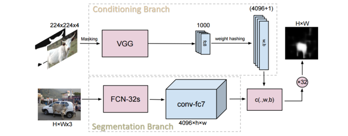
PASCAL VOC 2012 . - . - .

(mIoU) 40%, (31-33%). 2 (PSPNet, 83%).

11. Field-aware Factorization Machines in a Real-world Online Advertising System

: Yuchin Juan, Damien Lefortier, Olivier Chapelle, 2017
→ Original article
: Fedor Shabashev

Factorization machines CTR, , .

, .

, , .

, , factorization machines. factorization machine , ( naive).

CTR.
factorization machines - , . , .

, , , ( pre-mature).
.

12. The Marginal Value of Adaptive Gradient Methods in Machine Learning

: Ashia C. Wilson, Rebecca Roelofs, Mitchell Stern, Nathan Srebro, Benjamin Recht, 2017
→ Original article
: BelerafonL

: SGD, SGD+momentum, RMSProp, AdaGrad, Adam. – (RMSProp, Adam, AdaGrad) , SGD . , , .. SGD , – , .

SGD , . . , . - . . , SGD . , , learning rate decay, , , SGD. , , , , , …

13. FractalNet: Ultra-Deep Neural Networks without Residuals

: Gustav Larsson, Michael Maire, Gregory Shakhnarovich, 2016
→ Original article
: BelerafonL

, . FractalNet: Ultra-Deep Neural Networks without Residuals. , ResNet DenseNet. , , , , . .

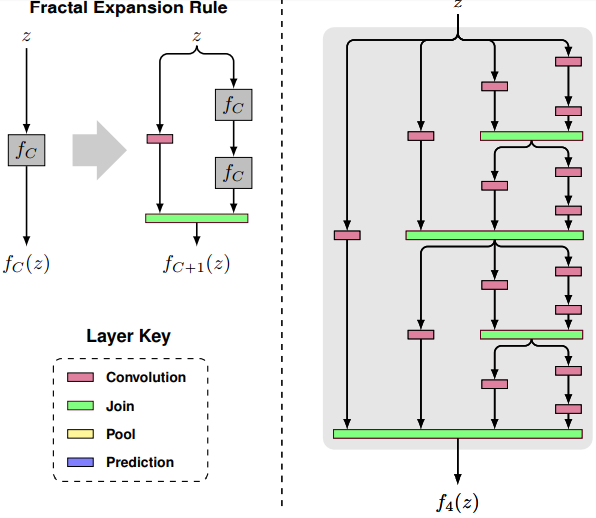
– . : . , . , , . , , . ResNet?

, Join ( ). , , , , - . . , . , . , , ,

, . Those. ( ) , , .

What does this give? , , .. , , , , , . Those. student-teacher.

, ResNet, , residual , FractalNet , . ResNet residual , – , residual . FractalNet , , .

, , , , ! ResNet, residual .

: « », .. . student-teacher , . 160 ( ) . ResNet (, ResNet ). – , , «» , residual. , , , . «» – .

:

, «» — .. col#4 , , .. . , , .. . , , «», , , .

, ResNet, . – , , , . Those. 3, – - . , – «» , .

, , 10 , .

, NIPS . ,
NIPS 2017 .