Probabilistic interpretation of classical machine learning models

In this article, I begin a series on generative models in machine learning. We will look at the classical tasks of machine learning, define what generative modeling is, look at its differences from the classical problems of machine learning, look at the existing approaches to solving this problem and dive into the details of those based on deep neural network training. But first, as an introduction, we look at the classical problems of machine learning in their probabilistic formulation.

Classic machine learning tasks

Two classic machine learning tasks are classification and regression. Let's look closer at each of them. Consider the formulation of both problems and the simplest examples of their solution.

Classification

The classification task is the task of labeling objects. For example, if objects are photographs, then the labels may be the content of the photographs: whether the image contains a pedestrian or not, whether the man or woman is depicted, what kind of dog is shown in the photograph. Usually there is a set of mutually exclusive labels and a collection of objects for which these labels are known. Having such a collection of data, it is necessary to automatically place labels on arbitrary objects of the same type that were in the original collection. Let's formalize this definition.
Suppose there are many objects . These can be points on a plane, handwritten numbers, photographs, or musical works. Suppose also that there is a finite set of labels . These tags can be numbered. We will identify the tags and their numbers. In this way in our notation will be denoted as . If a then the task is called a binary classification task; if there are more than two labels, then they usually say that it is just a classification task. Additionally, we have an input sample. . These are the very marked examples on which we will be trained to put labels automatically. Since we do not know the classes of all objects precisely, we consider that the class of an object is a random variable, which for simplicity we will also denote . For example, a photograph of a dog may be classified as a dog with a probability of 0.99 and as a cat with a probability of 0.01. Thus, in order to classify an object, we need to know the conditional distribution of this random variable on this object. .

Task of finding with a given set of tags and this set of tagged examples called the classification task.

Probabilistic formulation of the classification problem

To solve this problem, it is convenient to reformulate it in a probabilistic language. So, there are many objects and lots of tags . - a random variable representing a random object from . - a random variable representing a random label from . Consider a random variable with distribution which is the joint distribution of objects and their classes. Then, the marked sample is samples from this distribution. . We will assume that all samples are independently and equally distributed (iid in English literature).

The classification task can now be reformulated as the task of finding with this sample .

Classification of two normal distributions

Let's see how this works with a simple example. Set , , , , . That is, we have two gaussians, from which we are equally likely to sample the data and we need, having a dot from , predict from which Gaussian it was derived.

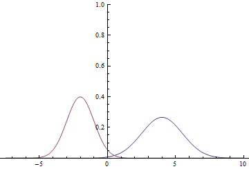
Fig. 1. Density distribution and .

Since the domain of the Gaussian is the entire numerical line, it is obvious that these graphs intersect, which means that there are such points at which the probability density and are equal.

Find the conditional probability of classes:

Those.

This is how the probability density graph will look like. :

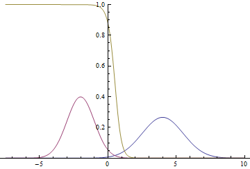
Fig. 2. Density of distribution , and . where two Gaussians intersect.

It can be seen that the confidence of the model in belonging to a particular class is very high (the probability is close to zero or one) is close to the Gaussian modes, and where the graphs intersect, the model can only guess by chance and give .

Likelihood Maximization Method

Most of the practical problems can not be solved as described above, since usually not explicitly set. Instead, there is usually a data set. with some unknown joint distribution density . In this case, the maximum likelihood method is used to solve the problem. The formal definition and justification of the method can be found in your favorite book on statistics or the link above, and in this article I will describe its intuitive meaning.

Likelihood maximization principle says that if there is some unknown distribution from which there is a set of samples and some well-known parametric family of distributions then in order to as close as possible , you need to find such a vector of parameters that maximizes the joint probability of data (likelihood) which is also called the likelihood of data. It is proved that under reasonable conditions this estimate is a consistent and unbiased estimate of the true vector of parameters. If samples are selected from , that is, iid data, then the joint distribution is decomposed into the product of the distributions:

Logarithm and multiplication by a constant are monotonically increasing functions and do not change the positions of the maxima, therefore the joint density can be introduced under the logarithm and multiplied by :

The last expression, in turn, is an unbiased and consistent estimate of the expected likelihood logarithm:

The maximization problem can be rewritten as a minimization problem:

The latter quantity is called the cross-entropy of the distributions. and . That is what is customarily optimized for solving learning problems with reinforcement (supervised learning).

Minimization throughout this cycle of articles will be carried out using the Stochastic Gradient Descent (SGD) , or rather, its expansion based on adaptive moments, using the fact that the sum of the gradients in the subsample (the so-called “mini-match”) is an unbiased estimate of the gradient of the minimized function.

Classification of two normal distributions by logistic regression

Let's try to solve the same problem that was described above, using the maximum likelihood method, taking as a parametric family simplest neural network. The resulting model is called logistic regression. The full model code can be found here , in the article only the key points are covered.

First you need to generate data for training. We need to generate a minibatch of class labels and for each label generate a point from the corresponding Gaussian:

def input_batch(dataset_params, batch_size): input_mean = tf.constant(dataset_params.input_mean, dtype=tf.float32) input_stddev = tf.constant(dataset_params.input_stddev,dtype=tf.float32) count = len(dataset_params.input_mean) labels = tf.contrib.distributions.Categorical(probs=[1./count] * count) .sample(sample_shape=[batch_size]) components = [] for i in range(batch_size): components .append(tf.contrib.distributions.Normal( loc=input_mean[labels[i]], scale=input_stddev[labels[i]]) .sample(sample_shape=[1])) samples = tf.concat(components, 0) return labels, samples 

We define our classifier. It will be the simplest neural network without hidden layers:

 def discriminator(input): output_size = 1 param1 = tf.get_variable( "weights", initializer=tf.truncated_normal([output_size], stddev=0.1) ) param2 = tf.get_variable( "biases", initializer=tf.constant(0.1, shape=[output_size]) ) return input * param1 + param2 

And we write the loss function - the cross-entropy between the distributions of real and predicted labels:

 labels, samples = input_batch(dataset_params, training_params.batch_size) predicted_labels = discriminator(samples) loss = tf.reduce_mean(tf.nn.sigmoid_cross_entropy_with_logits( labels=tf.cast(labels, tf.float32), logits=predicted_labels) ) 

Below are the graphs of learning of two models: basic and with L2 regularization:

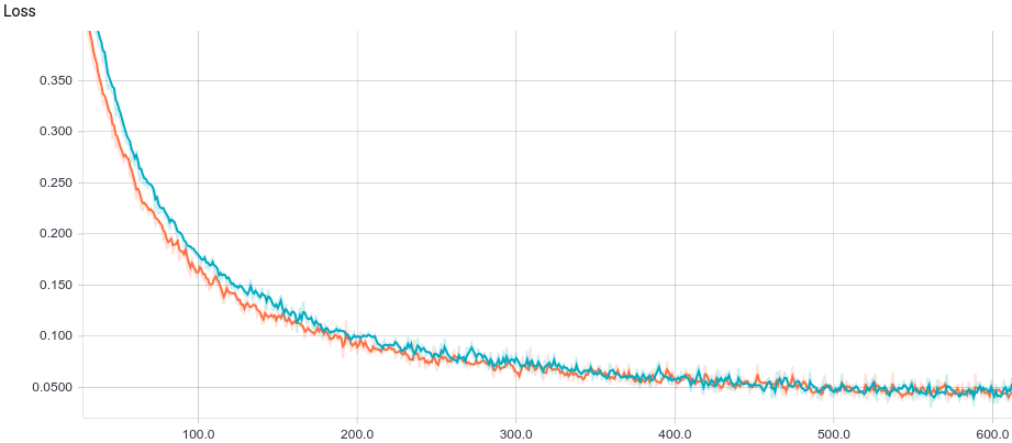
Fig. 3. Logistic regression learning curve.

It can be seen that both models quickly converge to a good result. The model without regularization performs better because in this problem regularization is not needed, and it slightly slows down the speed of learning. Let's take a closer look at the learning process:

Fig. 4. The process of learning logistic regression.

It can be seen that the trained dividing surface gradually converges to the analytically calculated one, and the closer it is, the slower it converges due to the increasingly weak gradient of the loss function.

Regression

The regression task is the task of predicting one continuous random variable. based on the values ​​of other random variables . For example, the prediction of a person’s height by gender (discrete random variable) and age (continuous random variable). In the same way as in the classification problem, we are given a marked sample. . Predicting the value of a random variable is directly impossible, because it is random and, in fact, is a function, therefore, formally, the task is written as a prediction of its conditional expected value:

Regression of linearly dependent quantities with normal noise

Let's see how the regression problem is solved with a simple example. Let there be two independent random variables . For example, this is tree height and normal random noise. Then we can assume that the age of the tree is a random variable . In this case, by linearity of expectation and independence and :

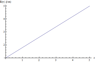
Fig. 5. The regression line of the problem is about linearly dependent values ​​with noise.

Solution of the regression problem with maximum likelihood method

Let's formulate the regression problem through the maximum likelihood method. Set ). Where - new parameter vector. We see that we are looking for - expected value i.e. This is the correct regression task. Then

A consistent and unbiased estimate of this expectation will be the average of the sample.

Thus, to solve the regression problem, it is convenient to minimize the root-mean-square error on the training set.

Regression of magnitude by linear regression

Let's try to solve the same problem as above, using the method from the previous section, taking as a parametric family the simplest possible neural network. The resulting model is called linear regression. The full model code can be found here , in the article only the key points are covered.

First you need to generate data for training. First we generate a minibatch of input variables. after which we get a sample of the original variable :

 def input_batch(dataset_params, batch_size): samples = tf.random_uniform([batch_size], 0., 10.) noise = tf.random_normal([batch_size], mean=0., stddev=1.) labels = (dataset_params.input_param1 * samples + dataset_params.input_param2 + noise) return labels, samples 

We define our model. It will be the simplest neural network without hidden layers:

 def predicted_labels(input): output_size = 1 param1 = tf.get_variable( "weights", initializer=tf.truncated_normal([output_size], stddev=0.1) ) param2 = tf.get_variable( "biases", initializer=tf.constant(0.1, shape=[output_size]) ) return input * param1 + param2 

And we write the loss function - L2-distance between the distributions of real and predicted values:

 labels, samples = input_batch(dataset_params, training_params.batch_size) predicted_labels = discriminator(samples) loss = tf.reduce_mean(tf.nn.sigmoid_cross_entropy_with_logits( labels=tf.cast(labels, tf.float32), logits=predicted_labels) ) 

Below are the graphs of learning of two models: basic and with L2 regularization:

Fig. 6. Linear regression learning curve.

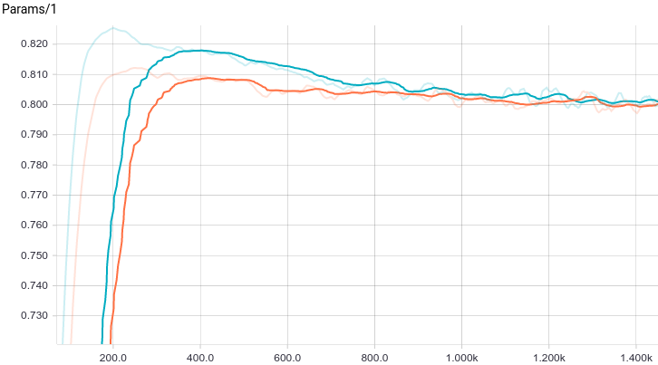
Fig. 7. Graph of the first parameter change with the learning step.

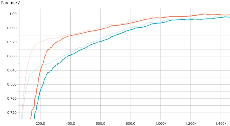
Fig. 8. Schedule of the second parameter change with a learning step.

It can be seen that both models quickly converge to a good result. The model without regularization performs better because in this problem regularization is not needed, and it slightly slows down the speed of learning. Let's take a closer look at the learning process:

Fig. 9. The process of learning linear regression.

It can be seen that the student expectation gradually converges to the analytically calculated one, and the closer it is, the more slowly it converges due to the increasingly weak gradient of the loss function.

Other tasks

In addition to the classification and regression problems studied above, there are other tasks of the so-called learning with a teacher, mainly reduced to the mapping between points and sequences: Object-to-Sequence, Sequence-to-Sequence, Sequence-to-Object. There is also a wide range of classic learning tasks without a teacher: clustering, filling data gaps, and, finally, explicit or implicit approximation of distributions, which is used for generative modeling. It is about the last class of problems that will be discussed in this series of articles.

Generative models

In the next chapter, we will look at what generative models are and how they differ fundamentally from the discriminative models discussed in this chapter. We look at the simplest examples of generative models and try to train a model that generates samples from a simple data distribution.

Thanks

Thank you Olga Talanova for reviewing this article. Thank you Sofya Vorotnikova for comments, editing and checking the English version. Thanks to Andrei Tarashkevich for the help in layout.