Welford method and multidimensional linear regression

Multidimensional linear regression is one of the fundamental methods of machine learning. Despite the fact that the modern world of data mining is captured by neural networks and gradient boosting, linear models still occupy an honorable place in it.

In previous publications on this topic, we learned how to obtain accurate estimates of averages and covariances using the Welford method, and then we learned how to apply these estimates to solve a one-dimensional linear regression problem. Of course, the same methods can be used in the multidimensional linear regression problem.

Linear models are often used due to several obvious advantages:

• high speed of learning and application;
• simplicity of models, which in many cases reduces the risk of retraining;
• the ability to build composite models using them: for example, having many hundreds of thousands of factors, you can train them in several linear models, the predictions of which can then be used as factors for more complex algorithms - for example, gradient boosting of trees.

In addition, there is another classic "advantage" of linear models, which is usually said about: interpretability. In my opinion, it is somewhat overvalued, but it is obvious that it is much easier to determine which sign has a characteristic coefficient in a linear model than to trace its use in a huge neural network.

Content

• 1. Multidimensional linear regression
• 2. General description of the solution
• 3. Application of the method of Welford
• 4. Implementation
• 5. Experimental comparison of methods
• Conclusion
• Literature

1. Multidimensional linear regression

In the multidimensional linear regression problem, it is required to recover the unknown dependence of the observed real value (which is the value of the unknown objective function ) $$$y ^ *$ from a set of real signs $$$f_1, f_2, ..., f_m$ .

Usually, for each individual observation, the values ​​of attributes and the objective function are recorded. Then from the values ​​of signs for all observations, you can make a matrix of signs $$$X$ , and from the values ​​of the objective function - the vector of its values $$$y$ :

$$

$$X_ {ij} = f_j (x_i), 1 \ leq i \ leq n, 1 \ leq j \ leq m$$

$$

$$y_i = y ^ * (x_i), 1 \ leq i \ leq n, 1 \ leq j \ leq m$$

Here $$$x_i$ - some specific observation. Thus, the rows of our matrix correspond to the observations, and the columns correspond to the features, and the total number of observations, and therefore rows in the matrix, $$$n$ .

For example, the target function may be the temperature value on a particular day. Signs - temperature values ​​in the previous days in geographically adjacent points. Another example is the prediction of a currency rate or a stock price; in the simplest case, again, the same value in the past can act as factors. A lot of observations are formed by calculating target values ​​and their corresponding attributes at different points in time.

Finding a solution to a problem means building some crucial function. $$$a: \ mathbb {R ^ m} \ rightarrow \ mathbb {R}$ . Now we are talking about the linear regression problem, so we will assume that the decision function is linear. In fact, this means that the decision function is simply the scalar product of the feature vector and some weight vector:

$$

$$a_ {w} (x_i) = \ sum_ {j = 1} ^ {m} w_j \ cdot f_j (x_i)$$

Therefore, the solution of our problem is the weight vector of signs $$$w = \ langle w_1, w_2, ..., w_m \ rangle$ .

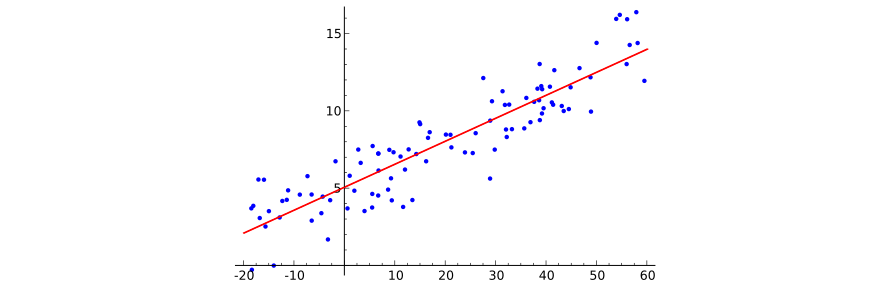
It is quite difficult to graphically represent a multidimensional linear relationship (for a start, let us imagine a 100-dimensional space of features ...), but the illustration for the one-dimensional case is quite enough to understand what is happening. Borrow this illustration from Wikipedia:

To complete the formulation of the machine learning problem, it is only necessary to indicate the loss functional, which answers the question how well a particular decision function predicts the values ​​of the objective function. Now we will use the root-mean-square loss functional traditional for regression analysis:

$$

$$Q (a, X, y) = \ sqrt {\ frac {1} {n} \ sum_ {i = 1} ^ {n} (a (x_i) - y_i) ^ 2}$$

So, the task of multidimensional linear regression is to find a set of weights. $$$w$ such that the value of the loss functional $$$Q (a_ {w}, A, y)$ reaches its minimum.

For analysis, it is usually convenient to abandon the radical and averaging in the loss functional:

$$

$$Q_1 (a, X, y) = \ sum_ {i = 1} ^ {n} (a (x_i) - y_i) ^ 2$$

For further presentation, it will be convenient to identify the observations with the sets of the corresponding factors:

$$

$$x_ {ij} = f_j (x_i)$$

It is easy to see that the loss functional is now simply written as a scalar square: the prediction vector can be written as $$$Xw$ , and the vector of deviations from the correct answers - as $$$Xw-y$ . Then:

$$

$$Q_1 (a, X, y) = \ langle Xw-y, Xw-y \ rangle$$

2. General description of the solution

It is well known from regression analysis that the solution vector in the multidimensional linear regression problem is found as a solution to a system of linear algebraic equations:

$$

$$(X ^ {T} X) w = X ^ {T} y$$

Proof of this is easy. Indeed, let's consider the partial derivative of the functional $$$Q_1$ by weight $$$j$ -th sign:

$$

$$\ frac {\ partial Q_1} {\ partial w_j} = 2 \ cdot \ sum_ {i = 1} ^ {n} (\ langle w, x_i \ rangle - y_i) \ cdot x_ {ij}$$

If we equate this derivative to zero, we get:

$$

$$\ sum_ {i = 1} ^ {n} (\ sum_ {k = 1} ^ {m} w_k \ cdot x_ {ik} - y_i) \ cdot x_ {ij} = 0$$

$$

$$\ sum_ {i = 1} ^ {n} \ Big (\ sum_ {k = 1} ^ {m} w_k \ cdot x_ {ik} \ cdot x_ {ij} \ Big) = \ sum_ {i = 1} ^ {n} x_ {ij} y_i$$

Now you can change the order of summation:

$$

$$\ sum_ {k = 1} ^ {m} w_k \ sum_ {i = 1} ^ {n} \ Big (x_ {ik} \ cdot x_ {ij} \ Big) = \ sum_ {i = 1} ^ { n} x_ {ij} y_i$$

Now it is clear that the coefficient at $$$w_k$ on the left is the corresponding element of the matrix $$$X ^ t x$ :

$$

$$\ sum_ {i = 1} ^ {n} (x_ {ik} x_ {ij}) = (X ^ {T} X) _ {jk}$$

In turn, the right side of the constructed equation is an element of the vector $$$X ^ t y$ :

$$

$$\ sum_ {i = 1} ^ {n} x_ {ij} y_i = (X ^ T y) _j$$

Accordingly, the simultaneous equalization of the partial derivatives with respect to all components of the solution to zero will lead to the desired system of linear algebraic equations.

3. Application of the method of Welford

When solving SLAE $$$(X ^ {T} X) w = X ^ {T} y$ Various problems arise, for example, the multicollinearity of features , which leads to the degeneracy of the matrix $$$(X ^ {T} X)$ . In addition, you must select a method to solve the specified SLAU.

I will not elaborate on these issues. Let me just say that in my implementation I use ridge regression with an adaptive choice of the regularization coefficient , and to solve the SLAE I use the LDL decomposition method.

However, now we will be interested in a much more mundane problem: how to form equations for a SLAE? If these equations are formed correctly, and the computational errors are small, one can hope that the chosen method will lead to a good solution. If errors have already appeared at the stage of forming the matrix of the system and the vector on the right side, no method for solving the SLAE will succeed.

From the above, it is clear that to compile a SLAE, it is necessary to calculate two types of coefficients:

$$

$$(X ^ TX) _ {kj} = \ sum_ {i = 1} ^ {n} (x_ {ik} x_ {ij})$$

$$

$$(X ^ Ty) _ {j} = \ sum_ {i = 1} ^ {n} (x_ {ij} y_i)$$

If the sample were centered, these would be expressions for the covariances mentioned in the very first article !

On the other hand, the sample can be centered independently. Let be $$$X '$ - matrix centered sample, and $$$y '$ - vector of answers for centered sampling:

$$

$$x '_ {ij} = x_ {ij} - \ frac {\ sum_ {k = 1} ^ {n} x_ {kj}} {n}$$

$$

$$y '_ {j} = y_ {j} - \ frac {\ sum_ {k = 1} ^ {n} y_k} {n}$$

Denote by $$$\ bar {x} _j$ average value $$$j$ th sign, and through $$$\ bar {y}$ - the average value of the objective function:

$$

$$\ bar {x} _j = \ frac {1} {n} \ sum_ {k = 1} ^ {n} x_ {kj}$$

$$

$$\ bar {y} = \ frac {1} {n} \ sum_ {k = 1} ^ {n} y_ {k}$$

Let the solution of the centered problem is the vector of coefficients $$$w '$ . Then for $$$i$ th event prediction value will be calculated as follows:

$$

$$a '(x') = \ sum_ {j = 1} ^ m {x'_j \ cdot w'_j} = \ sum_ {j = 1} ^ m {(x_j - \ bar {x} _j) \ cdot w'_j} = \ sum_ {j = 1} ^ m {x_j \ cdot w'_j} - \ sum_ {j = 1} ^ m {\ bar {x} _j \ cdot w'_j}$$

Wherein $$$a '(x')$ approximates centered value. From here we can finally write down the solution to the original problem:

$$

$$a (x) = \ sum_ {j = 1} ^ m {x_j \ cdot w'_j} - \ sum_ {j = 1} ^ m {\ bar {x} _j \ cdot w'_j} + \ bar { y}$$

Thus, linear regression coefficients can be obtained for the centered case using the formulas for calculating averages and covariances using the Welford method. Then they are trivially transformed into a solution for a non-centered case using the formula now derived: the coefficients of all attributes retain their values, while the free coefficient is calculated using the formula

$$

$$\ bar {y} - \ sum_ {j = 1} ^ m {\ bar {x} _j \ cdot w'_j}$$

4. Implementation

I put the implementation of multidimensional linear regression methods into the same program I spoke about last time .

When you first think about the fact that virtually the entire matrix of the multidimensional linear regression method is a large covariance matrix, you really want to make each of its elements a separate implementation of the class that implements the calculation of covariance. However, this leads to unjustified losses in speed: so, for each sign there will be $$$m$ times the average and sum of the weights are calculated. Therefore, as a result of thoughts, the next implementation was born.

The Welford multivariate linear regression problem solver is implemented as a TWelfordLRSolver class:

 class TWelfordLRSolver { protected: double GoalsMean = 0.; double GoalsDeviation = 0.; std::vector<double> FeatureMeans; std::vector<double> FeatureWeightedDeviationFromLastMean; std::vector<double> FeatureDeviationFromNewMean; std::vector<double> LinearizedOLSMatrix; std::vector<double> OLSVector; TKahanAccumulator SumWeights; public: void Add(const std::vector<double>& features, const double goal, const double weight = 1.); TLinearModel Solve() const; double SumSquaredErrors() const; static const std::string Name() { return "Welford LR"; } protected: bool PrepareMeans(const std::vector<double>& features, const double weight); }; 

Since in the process of updating the covariance values, we constantly have to deal with the differences between the current value of the attribute and its current average, as well as the average in the next step, it is logical to calculate all these values ​​in advance and add them into several vectors. Therefore, the class contains such a number of vectors.

When adding an element, the first thing to do is calculate the new vector of average values ​​of the signs and the magnitude of the deviations.

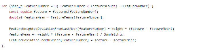
Already after this, the elements of the main matrix and the vector of the right parts are updated . From the matrix is ​​stored only the main diagonal and one of the triangles, because it is symmetrical.

Since the differences between the current values ​​of the factors and their averages are already calculated and stored in a special vector, the operation of updating the matrix turns out to be rather simple:

Saving on arithmetic operations here is more than justified, because This procedure of updating the matrix is ​​the most costly since. asymptotic CPU resources $$$O (m ^ 2)$ . Other operations, including update of the vector of the right parts are asymptotically linear:

The last element with the implementation of which it is necessary to understand is the formation of a decisive function. After the solution of the SLAE is received, it is converted to the original, non-centered, features :

 TLinearModel TWelfordLRSolver::Solve() const { TLinearModel model; model.Coefficients = NLinearRegressionInner::Solve(LinearizedOLSMatrix, OLSVector); model.Intercept = GoalsMean; const size_t featuresCount = OLSVector.size(); for (size_t featureNumber = 0; featureNumber < featuresCount; ++featureNumber) { model.Intercept -= FeatureMeans[featureNumber] * model.Coefficients[featureNumber]; } return model; } 

5. Experimental comparison of methods

Just as last time , implementations based on the Welford method ( welford_lr and normalized_welford_lr ) are compared with the "naive" algorithm, in which the matrix and the right side of the system are calculated using standard formulas ( fast_lr ).

I use the same dataset from the LIAC collection , available in the data directory. The same method of making noise in the data is used : the values ​​of the signs and responses are multiplied by a number, after which some other number is added to them. Thus, we can get a problem case from the point of view of computation: large average values ​​compared with the values ​​of the scatter.

In research-lr mode, the sample is changed several times in a row, and each time it runs a sliding control procedure. The result of the test is the average value of the coefficient of determination for test samples.

For example, for the kin8nm sample, the results of the work are obtained as follows:

 linear_regression research-lr --features kin8nm.features injure factor: 1 injure offset: 1 fast_lr time: 0.002304 R^2: 0.41231 welford_lr time: 0.003248 R^2: 0.41231 normalized_welford_lr time: 0.003958 R^2: 0.41231 injure factor: 0.1 injure offset: 10 fast_lr time: 0.00217 R^2: 0.41231 welford_lr time: 0.0032 R^2: 0.41231 normalized_welford_lr time: 0.00398 R^2: 0.41231 injure factor: 0.01 injure offset: 100 fast_lr time: 0.002164 R^2: -0.39518 welford_lr time: 0.003296 R^2: 0.41231 normalized_welford_lr time: 0.003846 R^2: 0.41231 injure factor: 0.001 injure offset: 1000 fast_lr time: 0.002166 R^2: -1.8496 welford_lr time: 0.003114 R^2: 0.41231 normalized_welford_lr time: 0.003978 R^2: 0.058884 injure factor: 0.0001 injure offset: 10000 fast_lr time: 0.002165 R^2: -521.47 welford_lr time: 0.003177 R^2: 0.41231 normalized_welford_lr time: 0.003931 R^2: 0.00013929 full learning time: fast_lr 0.010969s welford_lr 0.016035s normalized_welford_lr 0.019693s 

Thus, even a relatively small modification of the sample (scaling a hundred times with an appropriate shift) leads to the inoperability of the standard method.

In this case, the solution based on the method of Welford, is very resistant to poor data. The average operating time for the Welford method, thanks to all the optimizations, is only 50% longer than the average operating time for the standard method.

The only shame is that the "normalized" method of Welford also works poorly, and, moreover, it turns out to be the slowest.

Conclusion

Today we have learned how to solve a multidimensional linear regression problem, apply the Welford method in it, and make sure that using it allows us to achieve good accuracy of solutions even on “bad” data sets.

Obviously, if your task requires to automatically build a huge number of linear models and you do not have the opportunity to closely monitor the quality of each of them, and the additional execution time is not decisive, you should use the Welford method as yielding more reliable results.

Literature

1. habrahabr.ru: Exact calculation of averages and covariances by the Welford method
2. habrahabr.ru: Welford method and one-dimensional linear regression
3. github.com: Linear regression problem solvers with different computation methods
4. github.com: The Collection of ARFF datasets of the Connection Artificial Intelligence Laboratory (LIAC)
5. machinelearning.ru: Multidimensional linear regression