Flying snowflakes

1. Introduction

In heavily loaded portals or APIs, there may be a need to use machine learning algorithms, for example, to classify users. In the framework of this note, the process of implementation of some high-performance linear models will be shown, and explanations of the basic theoretical principles will be given.

2. Paired linear dependence

I will begin my story with the most frequently used and simple models. Suppose that there is a pair of metrics with a pronounced linear dependence. Visually display the data: the value of the first metric is the position of the point on the abscissa, and the value of the second metric is the position of the point on the ordinate. The figure shows that with an increase in the explanatory variable (it is also called a predictor, a regressor or an independent variable), an increase in the dependent variable occurs. For clarity, theoretical examples will be shown in R:

a <- c(1, 5, 5, 6, 4, 8, 9, 11, 15, 18, 22, 28, 29, 31, 31, 32) b <- c(1, 5, 6, 4, 5, 8, 9, 10, 17, 19, 22, 28, 28, 30, 30, 32) plot(a, b) abline(lm(b ~ a), col = "blue")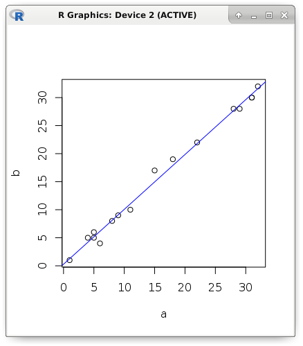 

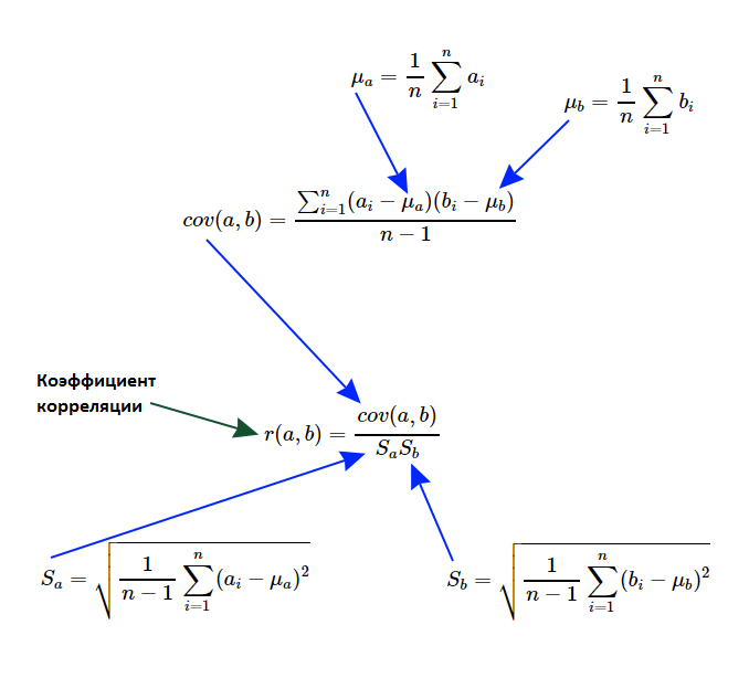
Let it be necessary to write such an algorithm, which should reveal the fact of the existence of a linear relationship, as well as measure its degree of expression. Formally speaking, it is necessary to calculate the linear correlation coefficient of Karl Pearson. I propose to recall the theoretical foundations and deal in more detail with the calculation formulas:

First of all, we are interested in such a characteristic of sets, which is called the variance of a random variable. If we take the average value from each element of the set and square the result, we get a new set, the average value of which is called the variance of the random variable for the general population. As you understand, if all the elements of the original set were the same, then the variance is zero, and the more the elements deviate from the average value, the greater will be the variance. And it can not be a negative number.

 var_a <- sum((a - mean(a)) ^ 2) / (length(a) - 1) c(var(a), var_a) # 127.2625 127.2625 c(sd(a), sqrt(var_a)) # 11.28107 11.28107 

Note that in the example shown above, we divided not by the power of the set, but by one less than it. In other words, we calculated the variance for the sample, not for the general population. And since the difference between the average and the element was squared, it now makes sense to extract the square root of the variance, thereby obtaining the standard deviation. To search for relationships, you need to know the standard deviation of the second set:

 var_b <- sum((b - mean(b)) ^ 2) / (length(b) - 1) c(var_b, var(b)) # 122.7833 122.7833 c(sd(b), sqrt(var_b)) # 11.08076 11.08076 

Now it is necessary to calculate such a measure of linear dependence of two quantities as covariance. The formula is very similar to variance, moreover, if the sets are identical, then we really get the variance of the random variable. The order of the arguments can be arbitrary (it is possible to interchange sets), since symmetry is visible by the formula - the covariance of A and B is equal to the covariance of B and A.

 cov_ab <- sum((a - mean(a)) * (b - mean(b))) / (length(a) - 1) c(cov(a, b), cov_ab) # 124.525 124.525 

Actually, the linear correlation coefficient of Karl Pearson is simply the ratio of the covariance and the product of the standard deviations of the sets. Unlike covariance, it is very convenient to interpret it: it is always in the range from -1 to 1. The closer it is to one, the higher the linear correlation. And proximity to -1 shows a negative correlation (in other words, the more one variable, the less the other). If it does not deviate strongly from zero, then this indicates a weak dependence. It is very important to emphasize that we are talking only about linear dependence without sharply pronounced outliers, otherwise the use of this coefficient will not make sense.

 cov_ab / (sqrt(var_a) * sqrt(var_b)) # 0.9961772 cor(a, b) # 0.9961772 

The linear correlation coefficient can be calculated after normalization or standardization of data, since the dependence will be preserved. Consider both the above mentioned modifications of the initial data - standardization and normalization. In the first case, the average value of each element of the set was subtracted (we got the force of deviation of this value from the average), and then we divided it by the standard deviation. As a result, we obtained a new set, in which the average value is 0, and the variance is 1. In the second case, we subtracted the minimum value from each element and divided it into a variational span (the data will be in the range from 0 to 1).

 #  nm <- function(a) { (a - mean(a)) / sd(a) } #  snt <- function(a) { (a - min(a)) / (max(a) - min(a)) } cor(a, b) # 0.9961772 cor(nm(a), nm(b)) # 0.9961772 cor(snt(a), snt(b)) # 0.9961772 

Observing a pairwise linear dependence, we approximate it by a straight line. This will make it possible to predict the value of one metric, if only the second is known. Since we are examining exactly the pairwise linear dependence, we should calculate only two parameters: a constant (intersection, offset, intercept) and the coefficient of the only predictor, i.e. slope of a straight line (slope). To calculate the predictor coefficient, it is enough to multiply the correlation by the result of dividing the standard deviation of the predictor and the dependent variable. The intersection can be found even easier: subtract from the average value of the predictor the result of the product of the coefficient and the average value of the dependent variable.

 slope <- cor(a, b) * (sd(b) / sd(a)) intercept <- mean(b) - (slope * mean(a)) c(intercept, slope) # 0.2803261 0.9784893 

If the dependency is not functional, but stochastic, then some error will appear. Consider an example. Let us try to predict the value of the dependent variable using linear regression if only the predictor is known. In red, I display the predicted values ​​that are strictly on the straight line, and the black ones - the actual value:

 y <- (0.2803261 + (0.9784893 * a)) plot(a, b) points(a, y, col = "red") abline(lm(b ~ a), col = "blue")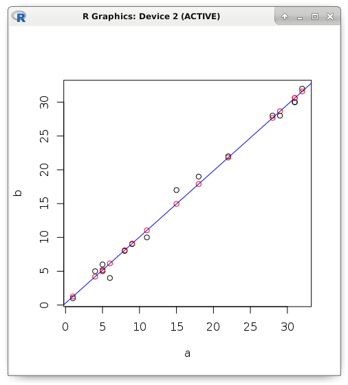 

Error is the difference between the actual and predicted value. For example, in the R programming language, descriptive error statistics are displayed in the Residuals clause. Robust (resistant to interference) measurement results are shown. The middle of the sorted set (median) is resistant to outliers (interference), as well as the lower or upper quartile. The average value is not used here because it is not resistant to emissions. It is not difficult to guess that the maximum and minimum are peculiar records (the most powerful mistake).

 summary(lm(b ~ a)) # Residuals: # Min 1Q Median 3Q Max # -2.15126 -0.61350 -0.09749 0.50744 2.04233 # # Coefficients: # Estimate Std. Error t value Pr(>|t|) # (Intercept) 0.28033 0.44308 0.633 0.537 # a 0.97849 0.02293 42.669 3.17e-16 *** # --- # Signif. codes: 0 '***' 0.001 '**' 0.01 '*' 0.05 '.' 0.1 ' ' 1 # 

In addition, the intercept and predictor coefficients that we calculated earlier are shown. Neighbor column is a standard error. The t-statistic is shown next to it, which tests the null hypothesis that the coefficient is zero (since there is no sense in subtracting zero from the coefficient, we simply divide the coefficient by the standard error). The level of significance is quite large, which allows you to reject the null hypothesis. For clarity, we calculate manually obtained indicators:

 e <- (b - y) # Residuals: c(min(e), quantile(e, .25), median(e), quantile(e, .75), max(e)) # -2.15126190 -0.61349440 -0.09748515 0.50744140 2.04233440 # Std. Error (a) sqrt(sum(e ^ 2) / ((length(e) - 2) * sum((a - mean(a)) ^ 2))) # 0.02293208 # t value (a) 0.9784893 / 0.02293208 # 42.66902 # Pr(>|t|) (a) round((pt(42.66902, df = 14, lower.tail = FALSE) * 2), digits = 18) # 3.17e-16 

Now we estimate the accuracy of the model using the following metrics: MSE, MAE and RMSE. The name MSE comes from the English Mean Square Error. This is the average square error. And the MAE (Mean Absolute Error) metric is the average absolute value of the error. In other words, in the first case we get the average value of the square of the error, and in the second - the average of the error modulus. The RMSE (Root Mean Square Error) metric is simply the square root of MSE.

 mae <- mean(abs(e)) mse <- mean(e ^ 2) rmse <- sqrt(mse) c(mae, mse, rmse) # 0.7131298 0.8783887 0.9372239 hist(e, breaks = 10, col = "blue")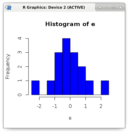 

3. Transferring existing models

Let us turn to a more practical aspect. Suppose that there is a very high-loaded API, in which you need to add functionality to detect the value of the dependent variable according to the value of the only predictor. In fact, we are talking about the problem of approximation (regression). The implementation of the linear function will differ in a very compact and high-performance code.

We assume that the API is written in PHP7. Let me remind you that the external system should not know anything about the principles of the model. All work logic will be encapsulated in one class. Only input requirements and return value are known. As the design strategy strategy suggests, the client will use any class that implements the interface. This interface will require the implementation of one method that takes a single argument (predictor), and returns a different scalar value - the dependent variable.

 <?php declare(strict_types = 1); interface IModel { /** * @param float $x * @return float */ public function predict(float $x): float; } class Example implements IModel { /** * @var float */ const SLOPE = 0.9784893; /** * @var float */ const INTERCEPT = 0.2803261; /** * @param float $x * @return float */ public function predict(float $x): float { return (self::INTERCEPT + (self::SLOPE * $x)); } } class Client { /** * @var IModel */ private $_model; /** * @param IModel $model */ public function setModel(IModel $model) { $this->_model = $model; } /** * @param float $x * @return float */ public function run(float $x): float { return $this->_model->predict($x); } } $client = new Client(); $client->setModel(new Example()); echo $client->run(17); 

For comparison, you can write a complete code for a pairwise linear relationship:

 <?php declare(strict_types = 1); class Model { /** * @var float */ public $slope = 0.0; /** * @var float */ public $intercept = 0.0; /** * @param array $x * @param array $y */ public function fit(array $x, array $y) { $this->slope = Stat::cor($x, $y) * (Stat::sd($y) / Stat::sd($x)); $this->intercept = Stat::mean($y) - ($this->slope * Stat::mean($x)); } /** * @param float $x * @return float */ public function predict(float $x): float { return ($this->intercept + ($this->slope * $x)); } } 

I implemented descriptive statistics methods in a separate class:

 <?php declare(strict_types = 1); class Stat { /** * @param array $values * @return float */ public static function max(array $values): float { return max($values); } /** * @param array $values * @return float */ public static function min(array $values): float { return min($values); } /** * @param array $values * @return float */ public static function sum(array $values): float { return array_sum($values); } /** * @param array $values * @return float */ public static function mean(array $values): float { return self::sum($values) / count($values); } /** * @param array $values * @return float */ public static function variance(array $values): float { $mean = self::mean($values); $pow = array_map(function($v) use ($mean) { return pow($v - $mean, 2); }, $values); return self::sum($pow) / (count($pow) - 1); } /** * @param array $values * @return float */ public static function sd(array $values): float { return sqrt(self::variance($values)); } /** * @param array $a * @param array $b * @return float */ public static function cov(array $a, array $b): float { $meanA = self::mean($a); $meanB = self::mean($b); $diff = []; for($i = 0; $i < count($a); $i++) { $diff[] = ($a[$i] - $meanA) * ($b[$i] - $meanB); } return self::sum($diff) / (count($diff) - 1); } /** * @param array $a * @param array $b * @return float */ public static function cor(array $a, array $b): float { return self::cov($a, $b) / (self::sd($a) * self::sd($b)); } } 

Let's complicate the task. Let the number of predictors be arbitrary. This is not a straight line, but a hyperplane in multidimensional space. And we change the type of the problem from approximation to classification. For example, the problem of binary classification was solved using logistic regression. We want to use this statistical model in our incredibly heavily loaded service, for example, to classify users. To solve the problem, we do not need the model learning algorithm itself, but only the parameters of the separating hyperplane.

In this situation, the principle of the model will remain the same. In the same way, the results of multiplying the predictors by their corresponding coefficients should be summed up. Then intercept is added to the amount received. Sometimes, instead of bias, an artificial constant predictor is added, then the whole formula will be reduced only to the sum of the predictor products with their coefficients (the scalar product of the weight vector and the feature vector).

For the classification problem, we simply compare the calculation result with a predetermined threshold. If the value is greater, then it is assigned the first class, otherwise - zero. The transfer of such a model will be identical. This is the two most important advantages of such linear models - compact code and very high performance. This allows literally on the fly to identify the class of observation on the vector of signs.

 #   dataset <- read.csv('dataset.csv') #      pairs(dataset, col = factor(dataset$class)) #     model <- glm(formula = class ~ ., data = dataset, family = binomial) #    b <- model$coefficients #    ,    nc <- (b[1] + (dataset$alpha * b[2]) + (dataset$beta * b[3])) > 0 plot(dataset$alpha, dataset$beta, col = factor(nc))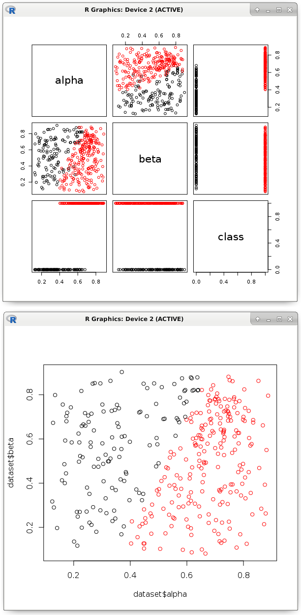 

The image shows that a similar linear function divided the points into two classes. Actually, its parameters and need to be exported to the code in another programming language. As we have seen, this is an easy task. This process is very well automated. The main thing is to be sure that such a hyperplane will correctly classify, and all predictors are really necessary.

Train the model and check its accuracy should be on different data sets. There are a number of classification accuracy metrics, the main ones we will definitely consider. First of all, I propose to recall the probability metric of an exact answer. It is calculated as the number of correct answers divided by the number of all answers.

 test <- factor(as.logical(dataset$class)) length(nc) # 345 table(test == nc) # FALSE TRUE # 17 328 328 / 345 # 0.9507246 

And what if the proportion of observations of one of the classes is only one thousandth of a percent? Here, even the constant issuing classifier will show a remarkable result. It makes sense to display the confusion matrix. In a binary classification, there can be only four outcomes of the prediction of a class label. A true positive result is the correct guessing of a positive class (TRUE is predicted to be TRUE). True negative - correct guessing of the negative class (FALSE predicted as FALSE). It is logical to assume that a false positive is FALSE predicted as TRUE, and a false negative is TRUE predicted as FALSE. Let's look at a specific example:

 table(nc, test) # test # nc FALSE TRUE # FALSE 120 8 # TRUE 9 208 

Where "nc" is the response of the classifier, and "test" is the true answer. Determine the proportion of positive responses of the classifier, which were really positive (accuracy, precision). As well as recall, i.e. what proportion of these positive ones could be identified by this model. The meaning of these indicators is the following: accuracy shows the degree of confidence in the classifier, if he gave a positive answer. In other words, as far as we can be sure that this is a really positive class. But the fullness shows the coverage of the detecting ability, i.e. share of positives identified. If we are afraid to mistakenly call a class positive, then accuracy is more important. When you need to find as many positive ones as possible, completeness is more important.

 library(caret) precision <- posPredValue(factor(nc), test, positive = T) # 0.9585253 recall <- sensitivity(factor(nc), test, positive = T) # 0.962963 #  F1       f1 <- (2 * precision * recall) / (precision + recall) # 0.960739 

Calculate manually the accuracy and completeness. It is enough to substitute values ​​from the confusion matrix:

 # precision ( /  + ) 208 / (208 + 9) # 0.9585253 # recall ( /  + ) 208 / (208 + 8) # 0.962963 

4. Assessing the importance of predictors

For example, a complex psychological study of people was carried out. One half of the subjects suffer from neurosis, while the other is doing well. What are the differences? Or another example: measured the performance of the equipment - some devices work well, but with others the problem. What influences it? Intuitively, we can assume that we should try to look for a correlation between the dependent variable and each of the predictors. Suddenly it turns out that, for example, the metric of fuel quality correlates strongly with durability (the better the fuel, the more durable the operation of the device). Or see the differences in the mean values ​​of predictors for observations of different classes.

However, let's try to visually display our data set. Some conditional border is visible, after which the dots change color. It passes in the region of 0.5 according to the alpha predictor. This can be seen in the histogram of its distribution (shown in different colors). And according to the “beta” predictor, there are no obvious differences.

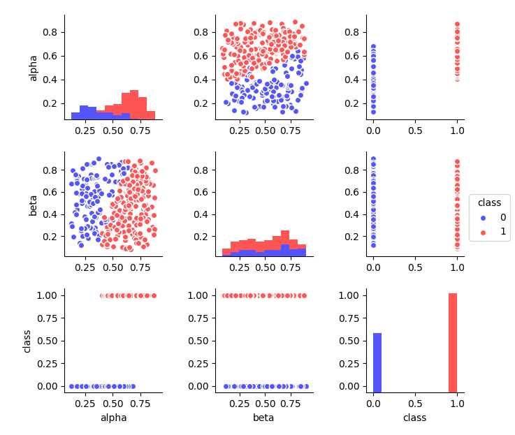
It is intuitively clear that, despite the error (some points will be incorrectly classified), such a criterion will more effectively solve the problem than any possible separation according to the “beta” predictor. Therefore, the importance of "alpha" will be quite high. After separation, the probability to meet the point of the desired class increases significantly. To identify the difference, we first calculate the probability without separation.

 table(dataset$class) # 0 1 # 129 216 length(dataset$class) # 345 c(129 / 345, 216 / 345) # 0.373913 0.626087 

Knowing the probabilities, we calculate the data homogeneity metric (if only representatives of one class, then the Gini impurity index will be equal to 0). Gini impurity is calculated as the sum of the squares of probabilities, which was taken from the unit.

 # Gini impurity gini <- function(p) { (1 - sum(p ^ 2)) } gini(c(0.373913, 0.626087)) # 0.4682041 

Divide all points by the condition mentioned earlier. The essence boils down to an intuitive logic: we want to choose the most effective separation according to the most informative predictor.

 node_1 <- subset(dataset, alpha > .5) table(node_1$class) # 0 1 # 25 197 length(node_1$class) # 222 #   gini(c(25/222, 197/222)) # 0.199862 

Repeat the procedure recursively with each new subset obtained. This will occur until a certain stopping condition, for example, until only observations of one class remain. This is well described by the decision tree, where in the nodes the corresponding test conditions (comparing the predictor with a constant) and in the terminal nodes (leaves) are observations of one class. Since the tree will try first of all to take the most effective predictors, the conditions of separation according to them will accumulate in the nodes close to the root. It turns out that the level (depth) of separation according to the predictor reflects its importance.

 node_2 <- subset(node_1, beta < .29) table(node_2$class) # 1 # 34 length(node_2$class) # 34 #      gini(c(0/34, 34/34)) # 0 

Agree that doing it manually is not the most comfortable task. This is where machine learning algorithms come to the rescue. Unfortunately, decision tree ensembles do not know how to explain (or rather, it is difficult to interpret a huge number of decision trees) the difference between classes, but they can calculate the importance of predictors. This also applies to approximation tasks, where the principle of operation is similar, only the separation criterion will be different.

On this dataset it was as clear as possible that one of the predictors has a very high significance. Let's see how it correlates with the class label:

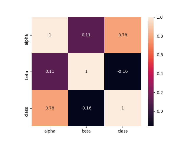
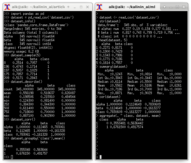
There are differences in the mean values ​​of different classes. I propose to look at descriptive statistics (examples in Python and R):

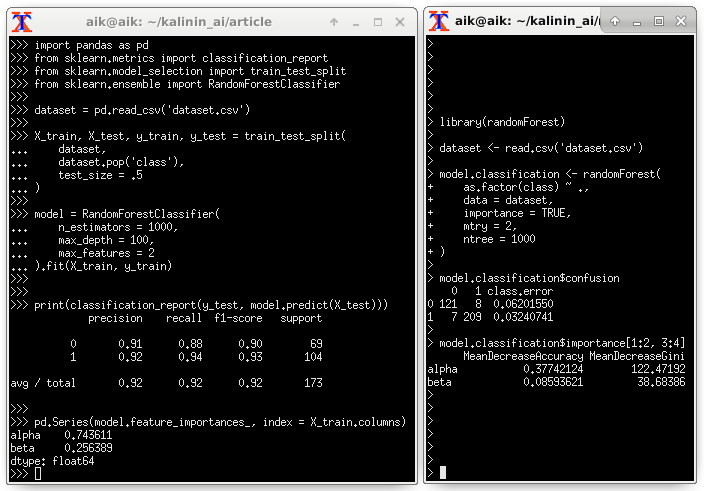
Assessing the importance of predictors through Random Forest:

5. Conclusions

The linear models described in the note have two main advantages that make it quite easy to transfer them to different projects. First, it is a compact code (only a few mathematical operations). Secondly, very high performance. However, everything has flaws. Unfortunately, if the points are poorly separated by a hyperplane or the dependence is poorly approximated by it, then the efficiency will be at an unacceptably low level.

6. Application

Used source code snippets (Python) to identify the degree of predictor importance:

 import pandas as pd dataset = pd.read_csv('dataset.csv') dataset.info() dataset.sample(5) dataset.describe() dataset.corr() dataset.groupby('class').mean() 

 import seaborn as sns import matplotlib.pyplot as plt dataset.hist(bins = 20, figsize = (6, 6)) plt.show() sns.heatmap(dataset.corr(), square = True, annot = True) plt.show() sns.pairplot( data = dataset, hue = 'class', size = 2, palette = 'seismic' ) plt.show() 

 import pandas as pd from sklearn.metrics import classification_report from sklearn.model_selection import train_test_split from sklearn.ensemble import RandomForestClassifier dataset = pd.read_csv('dataset.csv') X_train, X_test, y_train, y_test = train_test_split( dataset, dataset.pop('class'), test_size = .5 ) model = RandomForestClassifier( n_estimators = 1000, max_depth = 100, max_features = 2 ).fit(X_train, y_train) print(classification_report(y_test, model.predict(X_test))) pd.Series(model.feature_importances_, index = X_train.columns) 

 from catboost import CatBoostClassifier from sklearn.model_selection import KFold from sklearn.metrics import confusion_matrix, f1_score kf = KFold(n_splits = 3, shuffle = True) dataset = pd.read_csv('dataset.csv') y = dataset.pop('class').values X = dataset.values columns = dataset.columns for train_index, test_index in kf.split(X): X_train, X_test = X[train_index], X[test_index] y_train, y_test = y[train_index], y[test_index] model = CatBoostClassifier( calc_feature_importance = True ).fit(X_train, y_train) y_pred = model.predict(X_test) print(confusion_matrix(y_test, y_pred)) print(f1_score(y_test, y_pred)) print(list(zip(columns, model.feature_importances_)))