We teach the machine to understand the human genes
It is always pleasant to realize that the application of technology comes down not only to financial gain, there are also ideas that make the world a better place. We will tell about one of the projects with such an idea on this frosty Friday day. You will learn about the solution, which made it possible to increase the accuracy of rapid blood analysis, by using machine learning algorithms to identify the links between micro-RNA and genes. Also, it is worth noting that the methods described below can be used not only in biology.
We recently entered into a partnership agreement with Miroculus, a young promising company in the field of medical research. Miroculus is developing low-cost rapid blood test kits. As part of this project, we focused on the problem of identifying links between micro-RNA and genes by analyzing scientific and medical documentation, finding a solution that can be applied in many other areas.
The task of the Miroculus system is to identify the relationship of individual micro-RNA with certain genes or diseases. Based on these data, a tool is being developed and constantly improved, with the help of which researchers will be able to quickly identify the links between micro-RNA, genes and types of diseases (for example, oncological).
Although a lot of research is available in the medical literature regarding interdependencies between individual miRNAs, genes, and diseases, there is no single centralized database containing such information in an ordered structured form.
There can be various types of dependencies between micro-RNA and genes; however, due to lack of data, the problem of extracting connections has been reduced to binary classification, the purpose of which is simply to determine the connection between micro-RNA and the gene.
Detecting relationships between objects in unstructured text is called relationship retrieval .
Strictly speaking, the task receives unstructured text input data and a group of objects, and then displays the resulting group of triads of the form “first object, second object, type of connection”. That is, this is a subtask within the larger task of extracting information .
Since we are dealing with a binary classification, we need to create a classifier that receives a sentence and a pair of objects, and then displays the resulting score in the range from 0 to 1, reflecting the probability of a connection between these two objects.
For example, you can pass the sentence "mir-335 adjusts BRCA1" and a pair of objects (mir-335, BRCA1) to the classifier, and the classifier will give the result "0.9".
The source code for this project is available on the page .
We used the text of medical articles from two data sources: PMC and PubMed .
The text of documents downloaded from the indicated sources was divided into sentences using the TextBlob library.
Each proposal was transferred to the GNAT Object Recognition Tool to extract the names of micro-RNA and the genes contained in the proposal.
One of the most difficult tasks involved in retrieving relationships (or with basic machine learning tasks) is the availability of data with labels. In our project, such data was not available. Fortunately, we could use the “remote monitoring” method.
The term "remote monitoring" was first introduced in the study "Remote monitoring when extracting relationships without using data with tags" by Minz and co-authors. The method of remote observation involves the creation of a set of data with labels based on a database of known links between objects and a database of articles in which these objects are mentioned.
For each pair of objects and each link, link labels have been created in the database of objects for all sentences in the articles of the database where objects are mentioned.
To generate negative patterns (no link), we arbitrarily selected sentences containing links that are not displayed in the link database. It is worth noting that the main criticism of the method of remote observation is based on the possible inaccuracy of negative samples, since in some cases a false negative result can be obtained as a result of random sampling of data.
After creating a learning set with tags, a link qualifier is created using the scikit-learn Python library and several Python libraries based on natural language processing (NLP) technologies. As an experiment, we tried to use several different distinctive features and classifiers.
Before testing the methods and distinctive features in practice, we performed a text conversion consisting of the steps described below.
The idea is that the training model is not required in accordance with the name of a particular object, but it is necessary in accordance with the structure of the text.
Example:
Converting to:
That is, we practically took all the pairs of objects from each sentence and for each of them replaced the objects we were looking for with placeholders. At the same time, OBJECT1 always replaces micro-RNA, and OBJECT2 is always a gene. We also used another special placeholder to mark the objects that are part of the proposal, but do not participate in the desired connection.
So, for the following sentence:
we got the following set of converted sentences:
At this stage, you can use the Python method string.replace () if you want to replace objects, as well as the methods itertools.combinations or itertools.product, if you want to see all the possible combinations.
Markup is the process of splitting a sequence of words into smaller segments. In this case, we divide the sentences into words.
For this we use the nltk library:
In accordance with the recommendations presented in the scientific literature, we truncated each sentence to a smaller segment containing two objects, words between objects and a few words before and after the object. The purpose of this truncation is to remove those parts of the sentence that are not significant when extracting the relationship.
We created a slice of the array of words, for which the previous step was marked, providing it with appropriate indices:
We have normalized the sentences by simply converting all the letters to lowercase. Although it is advisable to use the case creation method for solving such tasks as analyzing moods and emotions, it is not indicative in terms of extracting relationships. We are interested in the information and structure of the text, and not the emphasis of individual words in the sentence.
In this case, we use the standard process of removing stop words and numbers from a sentence. Stop words are words with high frequency, for example, the prepositions "in," "to" and "to." Since these words are found in sentences very often, they do not carry a semantic load about the relationships between objects in a sentence.
For the same reason, we delete lexemes consisting only of numbers and short lexemes containing less than two characters.
Root extraction is the process of reducing a single word to the root.
As a result, the volume of semantic space for the word is reduced, which allows you to focus on the actual meaning of the word.
In practice, this step is not particularly effective in terms of improving accuracy. For this reason, and also because of the relatively low level of productivity of this process (in terms of execution time), the selection of roots was not included in the final model.
Normalization, deletion of words and selection of roots are performed by iterating the marked up and truncated sentences; if necessary, normalization and deletion of words is performed.
Upon completion of the transformations below, we decided to experiment with different types of distinctive features.
We used three types of signs: a multiset of words, syntactic signs and a vector representation of words.
The word set multiset (MS) model is a common method used in natural language processing (NLP) tasks for converting text into a numerical vector space.
In the MC model, each word in the dictionary is assigned a unique numeric identifier. Then each sentence is converted to a vector in the volume of the dictionary. The position in the vector is expressed by the value “1” in the event that the word with such an identifier is text, or the value “0” otherwise. As an alternative approach, you can customize the display in each element of the vector of the number of occurrences of a given word in the text. An example can be found here .
However, the model described above does not take into account the order of the various words in a sentence, but only the occurrence of each individual word. To include the word order in the model, we used the popular N-gram model, which evaluates a set of consecutive words of N words in length and treats each such set as a separate word.
For more information about using N-grams in textual analysis, see the section “Representation of distinctive features for textual analysis: one-gram, two-gram, trigram ... how much is all?”.
Fortunately for us, MC models and N-grams are implemented in scikit-learn by means of the CountVectorizer class.
The following example shows the conversion of text to the MS 1/0 view using a trigram model.
We used two types of syntactic features: markers of speech (PD) and parse trees with dependencies .
We decided to use spacy.io to extract both PD markers and dependency graphs, since this technology is superior to existing Python libraries in terms of speed, and accuracy is comparable to other NLP systems.
The following code snippet extracts the CR for the given sentence:
After converting all the sentences, you can use the CountVectorizer class described above and the multiset model for PD markers to convert them into a numeric vector space.
A similar method was used to process the distinguishing features of the parsing tree with the dependencies that were searched for between the two objects in each sentence, and they were also converted using the CountVectorizer class.
The method of vector representation of words has recently become very popular for solving problems related to NLP. The essence of this method is to use neural models to transform words into a space of distinctive features so that similar words are represented by vectors at a small distance from each other.
For more information about the vector representation of words, see the following blog article .
We applied the approach described in the Paragraph Vector document: embedding sentences (or documents) into a high-dimensional space of distinctive features. We used the Gensim implementation of the Doc2Vec library. More information is available in this tutorial .
Both the parameters and the size of the output vectors used correspond to the recommendations given in the Paragraph Vector document and the Gensim study guide.
Notice that in addition to tagged data, we used a large set of untagged sentences in the Doc2Vec model to provide additional context for the model and to expand the language and features used to train the model.
After creating the model, each of the proposals was represented by more than 200 dimensional vectors that can be used as input for the classifier.
Having completed the text conversion and extraction of distinctive features, you can proceed to the next step: the selection and evaluation of the classification model.
For classification, a logistic regression algorithm was used. We tried algorithms such as support vector machine and random forest, but the logistic regression showed the best results in terms of speed and accuracy.
Before proceeding to assess the accuracy of this method, it is necessary to divide the data set into a training set and a test set. To do this, simply use the train_test_split method:
This method divides the data set arbitrarily, with 75% of the data belonging to the training set, and 25% to the test set.
To train the classifier based on logistic regression, we used the scikit-learn LogisticRegression class. To assess the performance of the classifier, we use the classification_report class, which prints data on accuracy , return completeness and F1-Score for classification.
The following code snippet shows the logistic regression classifier training and the printout of the classification report:
An example of the result of executing the code fragment described above is as follows:
Note that the C parameter (it indicates the degree of regularization) is chosen arbitrarily for this example, but it must be configured using a cross validation check, as shown below.
We combined all the above methods and techniques and compared various distinctive features and transformations to select the optimal model.
We used the LogisticRegressionCV class to create a binary classifier with configurable parameters, and then analyzed another test suite to evaluate the performance of the model.
Please note that for simple and convenient testing of various parameters of different distinguishing features, you can use the GridSearch class.
The following table shows the main results of the comparison of various distinguishing features.
To check the accuracy of the model, the F1-Score scale was used, since it allows us to estimate both the accuracy and the completeness of the return to the model.
In general, it seems that when using a multiset of words in single-trigrams, maximum accuracy is ensured compared to other methods.
Although the Doc2Vec model is distinguished by maximum performance in determining the similarity of words, it does not guarantee decent results in terms of extracting relationships.
In this article, we looked at the method that was used to create a classifier for extracting relationships for processing links between micro-RNA and genes.
Although the problems and patterns discussed in this article are related to the field of biology, the solution and methods studied can be applied in other areas to create relationship graphs based on unstructured text data.
We remind you that you can try Azure for free .
Minute advertising . If you want to try new technologies in your projects, but do not reach the hands, leave the application in the program Tech Acceleration from Microsoft. Its main feature is that together with you we will select the required stack, we will help to realize the pilot and, if successful, we will spend maximum efforts so that the whole market will know about you.
 PS We thank Kostya Kichinsky ( Quantum Quintum ) for the illustration of this article.
Series of Digital Transformation articles
Technological articles:
1. Start .
2. Blockchain in the bank .
3. We learn the car to understand human genes .
4. Machine learning and chocolates .
5. Loading ...
')
A series of interviews with Dmitry Zavalishin on DZ Online :
1. Alexander Lozhechkin from Microsoft: Do we need developers in the future?
2. Alexey Kostarev from “Robot Vera”: How to replace HR with a robot?
3. Fedor Ovchinnikov from Dodo Pizza: How to replace the restaurant director with a robot?
4. Andrei Golub from ELSE Corp Srl: How to stop spending a lot of time on shopping trips?
We recently entered into a partnership agreement with Miroculus, a young promising company in the field of medical research. Miroculus is developing low-cost rapid blood test kits. As part of this project, we focused on the problem of identifying links between micro-RNA and genes by analyzing scientific and medical documentation, finding a solution that can be applied in many other areas.
Problem
The task of the Miroculus system is to identify the relationship of individual micro-RNA with certain genes or diseases. Based on these data, a tool is being developed and constantly improved, with the help of which researchers will be able to quickly identify the links between micro-RNA, genes and types of diseases (for example, oncological).
Although a lot of research is available in the medical literature regarding interdependencies between individual miRNAs, genes, and diseases, there is no single centralized database containing such information in an ordered structured form.
There can be various types of dependencies between micro-RNA and genes; however, due to lack of data, the problem of extracting connections has been reduced to binary classification, the purpose of which is simply to determine the connection between micro-RNA and the gene.
Detecting relationships between objects in unstructured text is called relationship retrieval .
Strictly speaking, the task receives unstructured text input data and a group of objects, and then displays the resulting group of triads of the form “first object, second object, type of connection”. That is, this is a subtask within the larger task of extracting information .
Since we are dealing with a binary classification, we need to create a classifier that receives a sentence and a pair of objects, and then displays the resulting score in the range from 0 to 1, reflecting the probability of a connection between these two objects.
For example, you can pass the sentence "mir-335 adjusts BRCA1" and a pair of objects (mir-335, BRCA1) to the classifier, and the classifier will give the result "0.9".
The source code for this project is available on the page .
Creating a dataset
We used the text of medical articles from two data sources: PMC and PubMed .
The text of documents downloaded from the indicated sources was divided into sentences using the TextBlob library.
Each proposal was transferred to the GNAT Object Recognition Tool to extract the names of micro-RNA and the genes contained in the proposal.
One of the most difficult tasks involved in retrieving relationships (or with basic machine learning tasks) is the availability of data with labels. In our project, such data was not available. Fortunately, we could use the “remote monitoring” method.
Remote surveillance
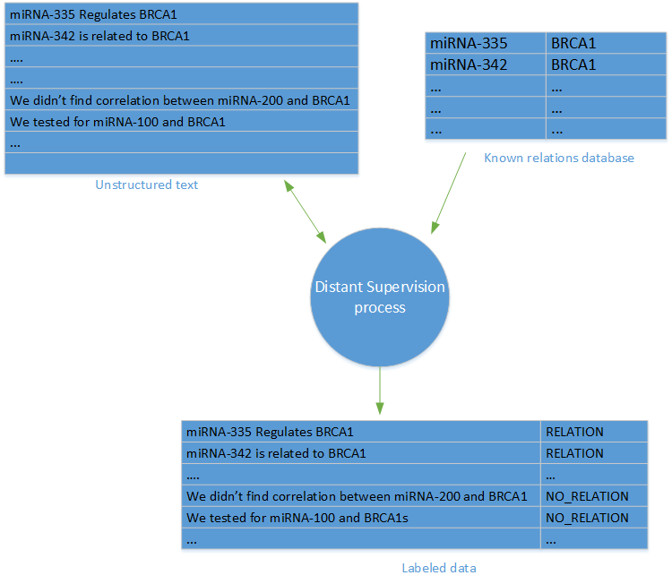
The term "remote monitoring" was first introduced in the study "Remote monitoring when extracting relationships without using data with tags" by Minz and co-authors. The method of remote observation involves the creation of a set of data with labels based on a database of known links between objects and a database of articles in which these objects are mentioned.
For each pair of objects and each link, link labels have been created in the database of objects for all sentences in the articles of the database where objects are mentioned.
To generate negative patterns (no link), we arbitrarily selected sentences containing links that are not displayed in the link database. It is worth noting that the main criticism of the method of remote observation is based on the possible inaccuracy of negative samples, since in some cases a false negative result can be obtained as a result of random sampling of data.
Text conversion
After creating a learning set with tags, a link qualifier is created using the scikit-learn Python library and several Python libraries based on natural language processing (NLP) technologies. As an experiment, we tried to use several different distinctive features and classifiers.
Before testing the methods and distinctive features in practice, we performed a text conversion consisting of the steps described below.
Object replacement
The idea is that the training model is not required in accordance with the name of a particular object, but it is necessary in accordance with the structure of the text.
Example:
miRNA-335 was found to regulate BRCA1 Converting to:
ENTITY1 was found to regulate ENTITY2 That is, we practically took all the pairs of objects from each sentence and for each of them replaced the objects we were looking for with placeholders. At the same time, OBJECT1 always replaces micro-RNA, and OBJECT2 is always a gene. We also used another special placeholder to mark the objects that are part of the proposal, but do not participate in the desired connection.
So, for the following sentence:
High levels of expression of miRNA-335 and miRNA-342 were found together with low levels of BRCA1 we got the following set of converted sentences:
High levels of expression of ENTITY1 and OTHER_ENTITY were found together with low levels of ENTITY2 High levels of expression of OTHER_ENTITY and ENTITY1 were found together with low levels of ENTITY2 At this stage, you can use the Python method string.replace () if you want to replace objects, as well as the methods itertools.combinations or itertools.product, if you want to see all the possible combinations.
Markup
Markup is the process of splitting a sequence of words into smaller segments. In this case, we divide the sentences into words.
For this we use the nltk library:
import nltk tokens = nltk.word_tokenize(sentence) Truncation
In accordance with the recommendations presented in the scientific literature, we truncated each sentence to a smaller segment containing two objects, words between objects and a few words before and after the object. The purpose of this truncation is to remove those parts of the sentence that are not significant when extracting the relationship.
We created a slice of the array of words, for which the previous step was marked, providing it with appropriate indices:
WINDOW_SIZE = 3 # make sure that we don't overflow but using the min and max methods FIRST_INDEX = max(tokens.index("ENTITY1") - WINDOW_SIZE , 0) SECOND_INDEX = min(sentence.index("ENTITY2") + WINDOW_SIZE, len(tokens)) trimmed_tokens = tokens[FIRST_INDEX : SECOND_INDEX] Normalization
We have normalized the sentences by simply converting all the letters to lowercase. Although it is advisable to use the case creation method for solving such tasks as analyzing moods and emotions, it is not indicative in terms of extracting relationships. We are interested in the information and structure of the text, and not the emphasis of individual words in the sentence.
Delete stop words / numbers
In this case, we use the standard process of removing stop words and numbers from a sentence. Stop words are words with high frequency, for example, the prepositions "in," "to" and "to." Since these words are found in sentences very often, they do not carry a semantic load about the relationships between objects in a sentence.
For the same reason, we delete lexemes consisting only of numbers and short lexemes containing less than two characters.
Root extraction
Root extraction is the process of reducing a single word to the root.
As a result, the volume of semantic space for the word is reduced, which allows you to focus on the actual meaning of the word.
In practice, this step is not particularly effective in terms of improving accuracy. For this reason, and also because of the relatively low level of productivity of this process (in terms of execution time), the selection of roots was not included in the final model.
Normalization, deletion of words and selection of roots are performed by iterating the marked up and truncated sentences; if necessary, normalization and deletion of words is performed.
cleaned_tokens = [] porter = nltk.PorterStemmer() for t in trimmed_tokens: normalized = t.lower() if (normalized in nltk.corpus.stopwords.words('english') or normalized.isdigit() or len(normalized) < 2): continue stemmed = porter.stem(t) processed_tokens.append(stemmed) Submission of distinctive features
Upon completion of the transformations below, we decided to experiment with different types of distinctive features.
We used three types of signs: a multiset of words, syntactic signs and a vector representation of words.
Multiset of words
The word set multiset (MS) model is a common method used in natural language processing (NLP) tasks for converting text into a numerical vector space.
In the MC model, each word in the dictionary is assigned a unique numeric identifier. Then each sentence is converted to a vector in the volume of the dictionary. The position in the vector is expressed by the value “1” in the event that the word with such an identifier is text, or the value “0” otherwise. As an alternative approach, you can customize the display in each element of the vector of the number of occurrences of a given word in the text. An example can be found here .
However, the model described above does not take into account the order of the various words in a sentence, but only the occurrence of each individual word. To include the word order in the model, we used the popular N-gram model, which evaluates a set of consecutive words of N words in length and treats each such set as a separate word.
For more information about using N-grams in textual analysis, see the section “Representation of distinctive features for textual analysis: one-gram, two-gram, trigram ... how much is all?”.
Fortunately for us, MC models and N-grams are implemented in scikit-learn by means of the CountVectorizer class.
The following example shows the conversion of text to the MS 1/0 view using a trigram model.
from sklearn.feature_extraction.text import CountVectorizer vectorizer = CountVectorizer(analyzer = "word", binary = True, ngram_range=(3,3)) # note that 'samples' should be a list/iterable of strings # so you might need to convert the processes tokens back to sentence # by using " ".join(...) data_features = vectorizer.fit_transform(samples) Syntactic features
We used two types of syntactic features: markers of speech (PD) and parse trees with dependencies .
We decided to use spacy.io to extract both PD markers and dependency graphs, since this technology is superior to existing Python libraries in terms of speed, and accuracy is comparable to other NLP systems.
The following code snippet extracts the CR for the given sentence:
from spacy.en import English parser = English() parsed = parser(" ".join(processed_tokens)) pos_tags = [s.pos_ for s in parsed] After converting all the sentences, you can use the CountVectorizer class described above and the multiset model for PD markers to convert them into a numeric vector space.
A similar method was used to process the distinguishing features of the parsing tree with the dependencies that were searched for between the two objects in each sentence, and they were also converted using the CountVectorizer class.
Vector representations of words
The method of vector representation of words has recently become very popular for solving problems related to NLP. The essence of this method is to use neural models to transform words into a space of distinctive features so that similar words are represented by vectors at a small distance from each other.
For more information about the vector representation of words, see the following blog article .
We applied the approach described in the Paragraph Vector document: embedding sentences (or documents) into a high-dimensional space of distinctive features. We used the Gensim implementation of the Doc2Vec library. More information is available in this tutorial .
Both the parameters and the size of the output vectors used correspond to the recommendations given in the Paragraph Vector document and the Gensim study guide.
Notice that in addition to tagged data, we used a large set of untagged sentences in the Doc2Vec model to provide additional context for the model and to expand the language and features used to train the model.
After creating the model, each of the proposals was represented by more than 200 dimensional vectors that can be used as input for the classifier.
Evaluation of classification models
Having completed the text conversion and extraction of distinctive features, you can proceed to the next step: the selection and evaluation of the classification model.
For classification, a logistic regression algorithm was used. We tried algorithms such as support vector machine and random forest, but the logistic regression showed the best results in terms of speed and accuracy.
Before proceeding to assess the accuracy of this method, it is necessary to divide the data set into a training set and a test set. To do this, simply use the train_test_split method:
from sklearn.cross_validation import train_test_split x_train, x_test, y_train, y_test = train_test_split(data, labels, test_size=0.25) This method divides the data set arbitrarily, with 75% of the data belonging to the training set, and 25% to the test set.
To train the classifier based on logistic regression, we used the scikit-learn LogisticRegression class. To assess the performance of the classifier, we use the classification_report class, which prints data on accuracy , return completeness and F1-Score for classification.
The following code snippet shows the logistic regression classifier training and the printout of the classification report:
from sklearn.linear_model import LogisticRegression from sklearn.metrics import classification_report clf = linear_model.LogisticRegression(C=1e5) clf.fit(x_train, y_train) y_pred = clf.predict(x_test) print classification_report(y_test, y_pred) An example of the result of executing the code fragment described above is as follows:
precision recall f1-score support 0 0.82 0.88 0.85 1415 1 0.89 0.83 0.86 1660 avg / total 0.86 0.85 0.85 3075 Note that the C parameter (it indicates the degree of regularization) is chosen arbitrarily for this example, but it must be configured using a cross validation check, as shown below.
results
We combined all the above methods and techniques and compared various distinctive features and transformations to select the optimal model.
We used the LogisticRegressionCV class to create a binary classifier with configurable parameters, and then analyzed another test suite to evaluate the performance of the model.
Please note that for simple and convenient testing of various parameters of different distinguishing features, you can use the GridSearch class.
The following table shows the main results of the comparison of various distinguishing features.
To check the accuracy of the model, the F1-Score scale was used, since it allows us to estimate both the accuracy and the completeness of the return to the model.
| Opportunities | F1-Score |
|---|---|
| Single-trigram (word set) | 0.87 |
| Single-trigrams (MC) and trigrams (markers CR) | 0.87 |
| Single-trigram (MS) and Doc2Vec | 0.87 |
| Odnograms (multiset of words) | 0.8 |
| Dvigrams (multiset of words) | 0.85 |
| Trigrams (multiset of words) | 0.83 |
| Doc2Vec | 0.65 |
| Trigrams (markers CR) | 0.62 |
In general, it seems that when using a multiset of words in single-trigrams, maximum accuracy is ensured compared to other methods.
Although the Doc2Vec model is distinguished by maximum performance in determining the similarity of words, it does not guarantee decent results in terms of extracting relationships.
Use cases
In this article, we looked at the method that was used to create a classifier for extracting relationships for processing links between micro-RNA and genes.
Although the problems and patterns discussed in this article are related to the field of biology, the solution and methods studied can be applied in other areas to create relationship graphs based on unstructured text data.
We remind you that you can try Azure for free .
Minute advertising . If you want to try new technologies in your projects, but do not reach the hands, leave the application in the program Tech Acceleration from Microsoft. Its main feature is that together with you we will select the required stack, we will help to realize the pilot and, if successful, we will spend maximum efforts so that the whole market will know about you.
PS We thank Kostya Kichinsky ( Quantum Quintum ) for the illustration of this article.Source: https://habr.com/ru/post/343604/
All Articles