Multi-channel attribution through Calltouch

Introduction

In recent years, the tools of a modern Internet marketer have been expanding at an ever faster pace. Today, in addition to search engine optimization (

$SEO$ ) and contextual advertising Yandex Direct and

$Google \: adwords$ in practical use entered

$e-mail$ channels, social networks,

$Instagram$ , remarketing / retargeting, etc. Therefore, the marketer is faced with the task of selecting those advertising channels that will be most effective for a particular project. Calltouch decided to talk about the fact that in addition to the difficulty of choosing the best advertising channels, it becomes quite difficult to comprehensively evaluate the effectiveness of a channel for the subsequent distribution of the advertising budget between them. Column Senior Product Manager Calltouch Fedor Ivanov mthmtcn .

According to Calltouch, this difficulty is primarily related to the fact that the user, for his part, has essentially the same tools as the marketer: he can come to the site either by direct link or by switching from social networks, from Yandex advertising and. etc. Moreover, before performing a target action (conversion) on a site, a user can repeatedly visit a site from different “entry points”: the first time he went to the site by clicking on an advertisement (

$CPC$ ), which Yandex issued on its search query, the second visit was on a direct transition (

$Direct$ ), well, and the third (resulting in conversion -

$C$ ) was from the social network (

$Social$ ) in this case we observe a chain (multichannel sequence):

$CPC → Direct → Social → C$

Thus, when evaluating the effectiveness of advertising channels, the marketer must first answer the question: how to evaluate the contribution of one or another source to the formation of conversion on the site? In another way, this question can be formed like this: what happens to the conversion on the site, if we exclude one or another marketing channel? To answer this question, there are a number of methodologies that are called attribution models. Consider these models in more detail.

')

Attribution models

An attribution model is a way to distribute the “weight” of conversion between channels. Depending on the choice of attribution model, the weight of the channel (source) will be calculated, which can be considered the contribution that this source has made to the conversion. Almost every user of Yandex Metrics or Google Analytics came across these models (section “multichannel sequences”). Currently, the following basic attribution models are distinguished:

By last interaction (last indirect interaction, last click on AdWords, last significant transition) - $Last \: Click \: Model \ :( LCM)$
The first interaction is $First \: Click \: Model \ :( FCM)$
Linear model - $Linear \: Model \ :( LM)$
Temporary decline - $Time \: Decay \: Model \ :( TDM)$
Based on position - $Position \: Type \: Model \ :( PTM)$

As already noted, the main difference between attribution models among themselves is a way to calculate the weight of a channel in a sequence. Consider each model in more detail. For clarity, we assume that we have the following multichannel sequence:

$$ display $$ AdWords → CPC → Social → E-mail → Yandex → CPC → Direct → C $$ display $$

Last Click Model

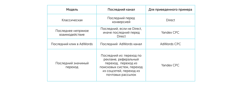
This model, due to its simplicity and intuitive "correctness", is most widely used in practice. In the most general case, within

$Lcm$ all models

$100%$ conversion weights are given to the last channel in a multichannel sequence, which preceded the fact of the occurrence of the target action. In our case, the classic

$Lcm$ model will give weight

$100%$ channel

$Direct$ and

$0%$ all other channels.

In practice, there are different varieties.

$Lcm$ models, they all differ from each other in how they choose the "last" channel. We present a table that demonstrates the method of channel selection depending on the type of model:

First Click Model

In this model

$100%$ weight is given to the first source in the sequence and

$0%$ everything else. In our case, the maximum weight will get the source

$Direct.$ If the model

$Lcm$ “Maximizes” the weight of the last channel, which “leads to action”, then

$FCM$ the model prefers the channel that starts the chain, that is, it “awakens the interest” of the user to the site. This model is also used in practice, although much less frequently than

$Lcm.$

Linear model

Linear model (

$LM$ ), as well as its generalizations and improvements (the model of temporary recession and on the basis of position) are united primarily by the fact that within its framework all the channels get their non-zero weight. The difference between the models is only in the way the weight is distributed between all the channels. When

$LM$ All channels get the same weight (that is, their contributions to the formation of a conversion) are considered equivalent. In our case, the channels

$AdWords \: CPC,$

$Social,$

$E-mail,$

$Yandex \: CPC,$

$Direct$ will have weight

$100/5 = $ 2$ %

Time decay

Attribution model

$TDM$ (

$Time \: Decay \: Model$ ) is based on the assumption that the contribution of the channel is greater, the more “closer” to the conversion it is, thus the weight of the channel is a monotonically increasing function of its position in the chain. The link can be found with the formula for calculating the weight of the channel.

Position Type Model

Attribution model

$PTM$ is a combination of three models:

$Lcm,$

$FCM$ and

$LM.$ Within its framework, the maximum share (usually by

$40%$ ) receive the first and last interactions in the chain, and the rest (usually

$20%$ a) evenly (as in the linear model) are distributed between the intermediate channels. In our example, the channels

$AdWords \: CPC$ and

$Direct$ will get by

$40%$ weights as well

$Social,$

$E-mail,$

$Yandex \: CPC$ by

$6.67%.$

How to choose an attribution model?

The choice of attribution model is the most important step in evaluating the effectiveness of advertising. Depending on the model, the analyst may receive absolutely opposite conclusions about the profitability of a channel. This is especially evident in the topics where the decision-making process takes a lot of time (for example, in real estate or in the automotive industry). A natural question arises: which attribution model should be taken as the standard? Unfortunately, there is no definitive answer to this question. Only a deep analysis of users' behavior on the site (user sessions) will allow us to make an informed decision on the choice of a particular method of linking conversions to the source of traffic.

As a rule, the choice stops on the model.

$Lcm,$ however, in practice, we have come across situations where

$Lcm$ on

$PTM$ With the subsequent distribution of funds between the channels, it was possible to significantly increase the effectiveness of marketing activities.

Separately, it is worth noting that the attribution model is the most important factor that should be taken into account when optimizing contextual advertising. Choosing a model directly affects the statistics used to calculate bids. If we assume that each key phrase is a separate advertising channel, then we can significantly enrich the statistics that go to the optimizer's input, in addition, the analysis of the user’s successive transitions between keywords will increase the optimization efficiency. A separate chapter of this work will be devoted to the discussion of this topic.

Before proceeding to the description of the approach used by us for the analysis of multichannel sequences, we give a “comic” example, which, on the one hand, will show the limitations of classical attribution models, and, on the other hand, allow us to formulate the basic questions that need to be answered.

Suppose the goal is C = "take the girl to his home to watch a movie . "

Suppose that we have the following chain of actions (essentially channels) that led to the desired goal:

Meet the girl → Invite to the cinema → Give flowers → Walk together in the park → Navigate to the house → Invite to a date in the restaurant → Give flowers → Dine for dinner → Drink a cocktail → Treat another cocktail → ... and another one → tell a joke → C

If we are dealing with a model

$Lcm,$ we believe that in order to achieve the goal we had, in principle, it was enough to get along with the anecdote. If you count within the model

$FCM,$ then success is guaranteed as soon as we met (which is more like the truth in comparison with the same anecdote). Model

$LM$ assumes that all actions have made an equal contribution. Model

$PTM$ It postulates that the fact of acquaintance and anecdote (and in equal shares) have the greatest contribution, while the influence of other factors is insignificant. Finally,

$TDM$ He believes that each of our next actions “warmed up” the interest of the girl, thereby increasing the likelihood of reaching the final goal, but still the anecdote was the decisive factor.

As we can see, none of the classical models can adequately describe the situation discussed above and, moreover, will not allow to correctly answer the question which channel (action) turned out to be the most important in reality.

We now formulate the main questions to which we would like to receive answers from the attribution model:

Is it enough just to tell a joke? And if so, how often?
How typical is the practice of telling anecdotes to achieve a goal?
What will happen if you do not tell a joke?
Is it possible to replace the anecdote with any other action? If so, which one should be replaced?

For the correct answer to most of the questions posed, it is not enough for us to consider only one sequence. It is required to collect some statistics that, on the one hand, would allow to predict the behavior of users, and on the other hand, would allow to estimate the probability of conversion on the site for each of the interaction points.

The model we are considering was originally developed for the cumulative evaluation of multichannel sequences, assuming that the channels are interdependent. It allows you to answer most of the questions formulated above. In addition, we will show how the methods described by us will allow us to predict the conversion rate for each key phrase, which is a necessary element in optimizing the rates in contextual advertising.

First of all, we describe the data format with which our model works.

User sessions

Suppose that for a certain period of time we analyze

$T$ , the site has been committed

$M$ transitions, that is, we have data about

$M$ user sessions. Each

$i$ session

$S_i$ has a fixed set of parameters (session attributes)

$P$ . For our analysis, we need the following set of attributes to be included in the set of all session attributes:

$A = \ {SrcType, \: TimeS, \: TimeF, \: URL, \: clientID, \: CVtype \} \ subset P,$

Where:

$SrcType$ - the channel through which the transition was made to the site
$Times$ - session start time
$Timef$ - session end time
$Url$ - the address of the page that the user got on going to the site
$clientID$ - unique user ID
$CVtype$ - whether the conversion was completed as a result of the session ( $CV$ - Yes, $N$ - not)

Further, for simplicity, we will assume that the time interval

$[TimeS; TimeF]$ is inside the analyzed period

$T$ , therefore we will remove attributes

$TimeS, \: TimeF$ from the considered set of parameters. It should also be noted that the parameter

$Url$ is required only to make the transition from the level of channels to the level of key phrases (subject to the presence of markup in

$Url$ ), which is useful for optimizing rates, but not necessarily for assessing the impact of channels on the conversion. By channel we understand the source of the traffic, which include:

Yandex CPC
Google CPC
Facebook
Vkontakte
Instagram
Direct
Referal
etc.

For simplicity, we will encode advertising channels as follows:

$c_1, \: c_2, \: ..., \: c_k$ , considering that their number is limited to

$k$ .

Now suppose that

$M$ sessions

$\ Sigma = \ {S_1, S_2, ..., S_M \}$ were initiated

$G \ leq M$ by users. With a unique user ID

$clientID$ can break many

$\ Sigma$ on

$G$ non-intersecting subsets:

$\ Sigma = U_1 \ cup U_2 ... \ cup U_G,$

Where

$U_i$ multiple sessions (sorted by increasing end date) with the same

$clientID$ , i.e., a plurality of sessions arranged in chronological order, initiated by the same user. Given our assumption that

$[TimeS; TimeF] \ subset T$ , then based on data in

$U_i$ we can match with everyone

$i$ The user has the following channel chain:

$c_ {i1} → c_ {i2} → ... → c_ {iL_i},$

Where

$L_i = | U_i |$ - the number of elements (in fact, the number of user transitions to the site) in the set

$U_i$ . The chain of conversions presented above is a sequence of traffic sources used

$i$ the user is in the process of interaction with the site.

We introduce two additional "pseudo-channel"

$CV$ and

$N$ according to the rule:

If during the session $i$ source user $c_ {ij} (1 \ leq j \ leq L_i)$ there was a conversion, then after $c_ {ij}$ add $CV$ by receiving $... → c_ {ij} → CV → ...$
If as a result of the last current session $i$ with source $c_ {iL_i}$ conversion did not happen then after $c_ {iL_i}$ add $N$ by receiving $... → c_ {iL_i} → N$

In addition, we also pay attention to the situation when we deal with chains of the form:

$... \ rightarrow c_ {ij} \ rightarrow CV \ rightarrow ... \ rightarrow CV \ rightarrow ...$

Sequences with such a structure cannot arise according to the rules formulated above, but nevertheless they can occur in a number of cases, for example, in calling topics, when in addition to the above session parameters we have a unique bundle:

$clientID → TelNumber$

In this case, the first call in the above chain will be a unique call, and all subsequent calls will be repeated calls of the subscriber with the specified

$clientID$ . Such chains will be taken into account in our model if, in addition to information about transitions to the site, there is a “log” of user interactions with the site, including offline (for example, the call log).

We note the key feature of the above method of forming chains of user interaction with the site. It lies in the fact that any interaction chain (multichannel sequence) always ends in one of two “events”:

$CV$ or

$N$ . With this event

$N$ can only occur at the end of the sequence, while

$CV$ may appear at any place.

We give typical examples of sequences formed according to the described rules. For simplicity, we limit ourselves to 3 different channels.

$c_1, \: c_2, \: c_3$ to which we add

$CV$ and

$N:$

$c_1 → N$
$c_1 → c_2 → N$
$c_1 → CV$
$c_1 \ rightarrow c_2 \ rightarrow CV \ rightarrow c_1 \ rightarrow N$
$c_1 \ rightarrow c_2 \ rightarrow CV \ rightarrow c_3 \ rightarrow N$
$c_1 → c_2 → CV → CV$
$c_1 \ rightarrow c_2 \ rightarrow CV \ rightarrow CV \ rightarrow c_3 \ rightarrow N$

The next step required to build a multichannel attribution model is to transform the sequences so that the event

$CV$ as

$N$ , could occur only strictly at the end of the sequence (such sequences will be called elementary). To do this, we will “split” the initial chains so that at the end they always stand

$CV$ or

$N$ .

Let us demonstrate this technique on the example of typical sequences:

chains 1-4 are already reduced to "elementary"
chain 5 "split" into: $c_1 → c_2 → CV$ and $c_1 → c_2 → c_1 → N$
chain 6 “split” into: $c_1 → c_2 → CV$ and $c_1 → c_2 → c_3 → N$
chain 7 “split” into: $c_1 → c_2 → CV$ and $c_1 → c_2 → CV$
chain 8 “split” into: $c_1 → c_2 → CV$ , $c_1 → c_2 → CV$ and $c_1 → c_2 → c_3 → N$

As a result of splitting, all the chains became “elementary”, and now we can proceed to the description of the model. However, before proceeding to this step, we already at this stage can answer the question: how to evaluate the effect of the channel on the conversion on the site.

Calculation of the influence of channels on the conversion

Consider a lot of

$G$ sequences (we will assume that all of them are already elementary, that is, they end in

$CV$ or

$N$ . Suppose that of sequences

$X$ end in

$CV$ and

$G$ -

$X$ on

$N$ . Denote the channel effect

$c_i$ for conversion on the site for a period of time

$T$ through

$I (c_i)$ , and elementary

$j$ chain through

$R_j$ . Size of influence

$I (c_i)$ channel

$c_i$ for conversion we will count as the number of “under-received” conversions in case of channel deletion

$c_i$ of all the conversion chains where it is present, referred to the total number of conversions

$X$ :

$I (c_i) = \ frac {| \ {R_j│c_i \ in R_j, \: CV \ in R_j \} |} {X}$

Obviously, for any

$c_i$ magnitude

$I (c_i)$ satisfies the following inequality:

$0 \ leq I (c_i) \ leq 1$

where

$I (c_i) = 0$ if and only if the channel

$c_i$ does not belong to any “conversion” sequence, and

$I (c_i) = 1$ if and only if deletion

$c_i$ will lead to the loss of all conversions on the site. Thus, it is easy to estimate the new number of conversions, which will be obtained after removing the channel

$c_i$ :

$CV_ {new} = X * (1-I (c_i))$

Calculate the effects of channels

$c_1$ ,

$c_2$ ,

$c_3$ for our example. Total we are seeing

$8$ conversions (conversion chains) of

$13$ elementary chains

$R_j$ . Channel

$c_1$ participates in all conversion chains, which means that its effect on conversion is

$1$ :

$I (c_1) = 1$ . Next, the channel

$c_2$ present in

$7$ conversion chains, which means

$I (c_2) = 7/8.$ Finally,

$c_3$ included in one conversion chain, then

$I (c_3) = 1 / 8.$

It is easy to replace that the sum of the channel effects is not equal to one. For convenience, you can enter the normalization and consider the normalized effect

$I_n (c_i)$ channels for conversion:

$I_n (c_i) = \ frac {I (c_i)} {\ sum \ limits_ {i = 1} ^ k I (c_i)}.$

In this case, obviously

$\ sum \ limits_ {i = 1} ^ k I_n (c_i) = 1.$

The formula for calculating the effect of the channel on the conversion can be easily modified for the case when you want to evaluate the effect of one channel on another. In particular, if the task is to find out how the channel affects

$c_i$ on

$c_j$ , you can use the following reasoning: user session initiated by the channel

$c_i$ leads to the channel session

$c_j$ as many times as there are chains

$R_f$ such that in them

$c_i$ preceded

$c_j$ . Then if we denote by

$I (c_i, c_j)$ the magnitude of this effect, then:

$I (c_i, c_j) = \ frac {| \ {R_f│c_i, c_j \ in R_t \: and \: c_i \: precede \: c_j \} |} {| \ {R_t│c_j \ in R_t \} |}.$

In the general case, the function

$I (c_i, c_j)$ not symmetrical:

$I (c_i, c_j) ≠ I (c_j, c_i).$ Sequences

$R_f$ such that they simultaneously

$c_i$ preceded

$c_j$ and

$c_j$ preceded

$c_i$ (i.e. cycles are formed) can also be taken into account in the denominator of the formula. The normalization introduced earlier is naturally generalized to the more general case just described:

$I_n (c_i, c_j) = \ frac {I (c_i, c_j)} {\ sum \ limits_ {h = 1} ^ k I (c_i, c_h)}.$

Estimate baseline metrics change when a channel is down

Answering the question how the number of conversions will change if you remove one or another channel from all chains

$c_i$ This raises the natural question of how the value of such basic metrics used in analyzing advertising effectiveness will change, such as:

consumption
cost of conversion (CPA)

It is quite difficult to answer these questions without attracting additional assumptions. Our basic axiom is that when a channel is deleted

$c_i$ from some chain

$R_j$ , the given chain is interrupted . More precisely, the wording looks like this: if the chain before the channel was deleted looked like:

$R_j = \ {c_ {i1} \ rightarrow c_ {i2} \ rightarrow ... \ rightarrow c_ {ik} \ rightarrow c_i \ rightarrow c_ {i (k + 1)} \ rightarrow ... \},$

then after removing the channel

$c_i$ the chain will be modified in:

$R_j \ rightarrow R_j ^ {new} = \ {c_ {i1} \ rightarrow c_ {i2} \ rightarrow ... \ rightarrow c_ {ik} \ rightarrow N \}.$

This assumption means that if you remove the channel that was used by the user to interact with the site, then there will be no further user interaction with this site.

To assess the base metrics, we also need to add in the parameters of user sessions such an indicator as “transition cost”. It can be interpreted as the cost that the advertiser pays for the user’s click on this channel, if the channel is free (such as a direct transition), then we assume that the transition cost is equal to

$0.$ If it is possible to establish only the total cost per channel (such as for

$SEO$ ), then we will assume that the cost of a transition in a particular session is equal to the ratio of the total cost per channel to the number of uses of this channel across all sessions. We will denote the cost of transition for the channel

$c_i$ in a chain

$R_j$ through

$V_j (c_i)$ . So we can estimate the cost

$V (r_j)$ single chain

$R_j$ in the following way:

$V (R_j) = \ sum \ limits_ {c_i \ in R_j} {V_j (c_i)}.$

At the same time, the total cost of the channel

$c_i$ are equal:

$V (c_i) = \ sum \ limits_ {j: c_i \ in R_j} {V_j (c_i)}.$

Total costs of attracting users to the site when using channels

$c_1, c_2, ..., c_k$ are equal:

$V = \ sum \ limits_ {j = 1} ^ G \ sum \ limits_ {c_i \ in R_j} {V_j (c_i)} = \ sum \ limits_ {i = 1} ^ k \ sum \ limits_ {j: c_i \ in R_j} {V_j (c_i)}.$

The duality of the formula is explained by different ways of calculating total costs: in the first case, we summarize the costs of each of the chains over all

$G$ chains, and in the second we summarize the cost of the channel for all

$k$ channels.

To estimate new costs after deleting from all chains of the channel

$c_i$ It seems most obvious to use the formula:

$V_ {new} = V_ {old} - \ sum \ limits_ {j: c_i \ in R_j} {V (R_j)},$ Where

$V_ {new}$ - new flow after channel removal

$c_i$ , but

$V_ {old}$ - former consumption. However, such simple logic does not lead to a correct estimation of costs, for the reason that in those chains

$R_j$ where meets

$c_i$ , other non-remote channels could be involved before it. Thus, for a more accurate estimate, we need to consider the value of the "truncated" chains. Therefore:

$V_ {new} = V_ {old} - \ sum \ limits_ {j: c_i \ in R_j} \ sum \ limits_ {t: \: c_t \: precede \: c_i} {V_j (c_t)}.$

It's obvious that

$\ sum \ limits_ {j: c_i \ in R_j} \ sum \ limits_ {t: \: c_t \: precede \: c_i} {V_j (c_t)} <\ sum \ limits_ {j: c_i \ in R_j} { V (R_j)},$

which means

$V_ {old} -V (c_i) <V_ {old} - \ sum \ limits_ {j: c_i \ in R_j} \ sum \ limits_ {t: \: c_t \: precede \: c_i} {V_j (c_t) }.$

The last inequality means that removing any channel

$c_i$ usually leads to the emergence of new chains with a certain value, which obviously will not bring conversions. So we can estimate the loss

$Loss (c_i)$ from the removal of the channel (the cost of all the "truncated" chains), as well as the savings

$EC (c_i)$ as the cost of all “unimportant” transitions that would have occurred if the channel were kept in chains:

$Loss (c_i) = \ sum \ limits_ {j: c_i \ in R_j} \ sum \ limits_ {t: \: c_t \: precede \: c_i} {V_j (c_t)},$

$EC (c_i) = \ sum \ limits_ {j: c_i \ in R_j} {V (R_j)} - Loss (c_i).$

Now, after we learned to evaluate the cost change after deleting a channel

$c_i$ , we can estimate the new cost of conversion, which would have occurred if there was no channel:

$CPA_ {new} = \ frac {V_ {new}} {CV_ {new}} = \ frac {V_ {old} - \ sum \ limits_ {j: c_i \ in R_j} \ sum \ limits_ {t: \: c_t \: precede \: c_i} {V_j (c_t)}} {X * (1-I (c_i))$

If we assume that prior to deleting the channel, we had the same conversion cost:

$CPA_ {old} = \ frac {V_ {old}} {X}$

and the goal of removing a channel is to reduce the cost of conversion, the decisive rule may be as follows:

$CPA_ {new} -CPA_ {old} <0.$

That is, if deleting a channel leads to a decrease in the cost of conversion (with a reasonable decrease in their number), then it can be excluded from the chains and stop spending the budget on it.

In addition, you can estimate the cost of “under-received conversions” when deleting a channel:

$CPA_ {loss} = \ frac {V_ {old} -V_ {new}} {X * I (c_i)},$

so instead of the rule

$CPA_ {new} -CPA_ {old} <0$ you can use another: if the relation is satisfied

$CPA_ {loss}> CPA_ {old},$

then delete the channel

$c_i$ will reduce the total cost of conversion on the site.

We now proceed to the description of the basic model required to calculate the probability of channel conversion.

Model Description

Before we begin to describe the multi-channel attribution model, we would like to refer to the excellent articles by Sergey Bryl, and the second article , in which the author used the beauty and functionality of Markov chains to describe multi-channel attribution. In this article, we described in more detail the main points related to the calculation of the probability of conversion in the framework of Markov processes, and also proposed an effective method for calculating the probability of conversion - based on stochastic matrices.

We will offer two alternative interpretations of the multi-channel attribution model: graph and matrix. The first will allow you to visually describe the model, while the second allows you to effectively calculate the required characteristics. We show that both descriptions actually represent the same random process, which is called a Markov process, and the model corresponding to the process represents a Markov chain.

Graph model

A graph is an abstract mathematical object representing a set of vertices of a graph and a set of edges, that is, connections between pairs of vertices. For example, for a lot of peaks, you can take a lot of airports served by some airline, and for a lot of ribs you can take regular flights of this airline between cities.

A graph is said to be oriented if each of its edges has a direction, i.e., in essence, is a vector: for an edge, it is precisely indicated which vertex it comes from, and in which it ends.

A graph is called weighted if a certain numerical value, called a weight, is assigned to its each edge. A typical example of a weighted oriented graph is a network of highways between cities (graph vertices), where by the weight of an edge (road) we mean its length.

In order to represent the set of chains as a graph, we need to fix two sets: the set of vertices

$V$ and many connections

$E$ between them. In the role of peaks will be the marketing channels as well as two additional events:

$V = \ {c_1, \: c_2, \: ..., \: c_k, \: CV, \: N \}.$

$E$ choose pairs of interconnected elements from

$V$ . For the above elementary chains we have:

$V = \ {c_1, \: c_2, \: c_3, \: CV, \: N \}, \\ E = \ {(c_1, N), \ :( c_1, c_2), \ :( c_2, N), \ :( c_1, CV), \ :( c_1, c_2), \: ..., \ :( c_3, N) \}.$

In view of the fact that in the set

$E$ there can be coinciding elements, the resulting graph can have multiple (duplicated) edges.

As can be seen, even for a small number of sessions such a graphical representation is rather cumbersome, which complicates the analysis. Some simplification can be achieved by replacing duplicated edges with one edge, taking the number of duplicates by weight. Then the original graph is converted to a weighted oriented graph:

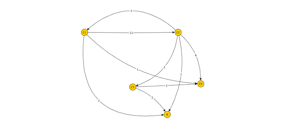
This graph is more suitable for analysis. Our next goal is to convert the edge weight to probabilistic notation. Replace the weight of the edge connecting the two vertices, the probability of transition from one vertex to another.

In particular, consider the top

$c_1$ . The following vertices of the graph are reachable from it:

$c_2, \: CV, \: N$ . Just from the top

$c_1$ was fixed

$1 + 11 + 2 = 14$ transitions, and

$11$ of them were in

$c_2$ ,

$2$ - at

$N$ and one in

$CV$ . Then if you mark

$P (c_1, c_2), \: P (c_1, N), \: P (c_1, CV)$ - probabilities to jump out

$c_1$ at

$c_2, \: CV, \: N$ respectively, then:

$P (c_1, c_2) = \ frac {11} {14}, \: P (c_1, N) = \ frac {2} {14} = \ frac17, \: P (c_1, CV) = \ frac { 1} {14}.$

Easy to replace that

$P (c_1, CV)$ - is the probability of source conversion

$c_1$ in the classic model

$Lcm.$ It becomes obvious that the model

$Lcm$ does not take into account the large amount of statistical data that we can collect by analyzing user sessions. If we make calculations for all remaining vertices, then our graph will be converted to the form:

Based on this model, you can calculate the total probability of conversion for a particular channel. The following recursive formula is used for the calculation:

$P_ {full} (c_i, CV) = \ sum \ limits_ {c_j: c_i \ rightarrow c_j} {P (c_i, c_j) P_ {full} (c_j, CV)}$

The meaning of this formula is that in order to calculate the total probability of converting a certain vertex, you need to select all the vertices reachable from a given one, then calculate the probabilities of transition to these vertices from the original, and then for each reachable vertex, again calculate the total probability of conversion. This formula immediately gives the full probability of conversion if the graph is unidirectional, that is, if there is an edge connecting the vertices

$c_i$ and

$c_j$ but missing edge that connects

$c_j$ c

$c_i$ . Otherwise, the above formula defines a system of linear equations, the number of unknowns in which is equal to the number of “returnable” edges in the graph.

For example, we calculate the total probability of conversion.

$P_ {full} (c_1, CV)$ for source

$c_1$ .

Because

$c_1$ associated with

$c_2, \: CV, \: N$ but the probability of moving from

$N$ at

$CV$ equals zero, and the probability of transition from

$CV$ at

$CV$ equals 1, then:

$P_ {full} (c_1, CV) = P (c_1, c_2) * P_ {full} (c_2, CV) + P (c_1, CV) * 1 = \ frac {11} {14} * P_ {full} (c_2, CV) + \ frac {1} {14}.$

In turn from

$c_2$ you can return to

$c_1$ or go to

$c_3, \: CV, \: N$ , which means:

$P_ {full} (c_2, CV) = P (c_2, c_1) * P_ {full} (c_1, CV) + P (c_2, c_3) * P_ {full} (c_3, CV) + P (c_2, CV ) * 1, \\ P_ {full} (c_2, CV) = \ frac {1} {11} * P_ {full} (c_1, CV) + \ frac {3} {11} * P_ {full} (c_3 , CV) + \ frac {6} {11},$

then

$P_ {full} (c_1, CV) = \ frac {11} {14} * \ Bigl (\ frac {1} {11} * P_ {full} (c_1, CV) + \ frac {3} {11} * P_ {full} (c_3, CV) + \ frac {6} {11} \ Bigr) + \ frac {1} {14}.$

For convenience, we denote

$P_ {full} (c_1, CV) = x$ , then we get the following linear equation:

$x = \ frac {11} {14} * \ Bigl (\ frac {1} {11} * x + \ frac {3} {11} * P_ {full} (c_3, CV) + \ frac {6} { 11} \ Bigr) + \ frac {1} {14}.$

Now let's calculate

$P_ {full} (c_3, CV)$ . From the source

$c_3$ can only go to

$CV$ or

$N$ . Then

$P_ {full} (c_3, CV) = \ frac {1} {3}.$

Finally we have the following equation:

$x = \ frac {11} {14} * \ Bigl (\ frac {1} {11} * x + \ frac {3} {11} * \ frac {1} {3} + \ frac {6} {11 } \ Bigr) + \ frac {1} {14}.$

From where

$x = P_ {full} (c_1, CV) = \ frac {8} {13} = 0.6154.$

.

The main advantage of the above model is its visibility, while obvious shortcomings (as can be seen even by a simple example) include high computational complexity for the case of a large number of traffic sources. Moreover, if different keywords are used as sources, the amount of calculations will increase by orders of magnitude, which will make all subsequent calculations unworkable. In addition, if we assume the possibility of transitions in the column of the form:

$... \ rightarrow c_i \ rightarrow c_i \ rightarrow ...$ (that is, allow loops), then the system of equations becomes nonlinear, which makes it much more difficult to find the required probabilities. In the next section, we turn to the consideration of the matrix model and show effective methods for calculating total probability formulas.

Matrix model

In the previous chapter, we looked at the graph model of multi-channel attribution. In order to convert it to a more convenient form for calculations, we again consider a set of

$k$ channels

$c_1, c_2, ... c_k$ and two additional "pseudo channels"

$CV$ ,

$N$ . I recall that in the graph model, they played the role of vertices.

According to the observed sequences compiled for each user, we can easily calculate the transition probabilities (in other words, conditional probabilities)

$P (c_i, c_j), \: P (c_i, CV), \: P (c_i, N)$ . As noted earlier, we will assume that

$P (N, c_i) = P (CV, c_i) = 0$ and

$P (N, N) = P (CV, CV) = 1$ . Then you can make a square matrix of size

$(k + 2) \ times (k + 2)$ whose elements are conditional probabilities

$P (c_i, c_j), \: P (c_i, CV), \: P (c_i, N), \: P (N, c_i), \: P (CV, c_i):$

and

$P (N, N), \: P (CV, CV)$ :

$H = \ begin {pmatrix} P (c_1, c_1) & P (c_1, c_2) & ... & P (c_1, c_k) & P (c_1, CV) & P (c_1, N) \\ P (c_2, c_1)& P(c_2,c_2)& …& P(c_2,c_k)& P(c_2,CV) & P(c_2,N) \\ …&…&…&…&…&… \\ P(c_k ,c_1) & P(c_k,c_2) & … & P(c_k,c_k) & P(c_k,CV) & P(c_k,N) \\ 0&0&…&0&1&0 \\ 0&0&…&0&0&1 \end{pmatrix}$

In particular, for the example considered above, we obtain:

$H=\begin{pmatrix} 0&\frac{11}{14}&0&\frac{1}{14}&\frac{2}{14}\\ \frac{1}{11}&0&\frac{3}{11}&\frac{6}{11}&\frac{1}{11}\\ 0&0&0&\frac13&\frac23\\ 0&0&0&1&0\\ 0&0&0&0&1 \end{pmatrix}$

It is easy to notice that for any

rows of matrix

$i$

holds true:

$H$

$\sum\limits_{j=1}^k{P(c_i,c_j)}+P(c_i,CV)+P(c_i,N)=1.$

The matrix for which this condition is satisfied is called stochastic. It is known that an arbitrary stochastic matrix defines a random process called Markov. Let us give such a process a more formal (although not rigorous from a mathematical point of view) definition.

A Markov process is such a random process with a certain number of states that the probability of transition to the next state depends only on the current state in which the system is located.

Thus, the process of transitions between different marketing channels that we are considering can be considered a Markov process defined by a matrix of transition probabilities.

$H$ . The model thus defined makes it possible to answer a number of important questions, in particular:

What is the probability of transition from the state to state $c_i$ $c_j$ behind steps? $t$
How will the probability distribution of finding in each of the channels through steps? $t$

In our applied problem of estimating the probability of conversion of each channel, we need to answer a particular case of the first question:

What is the total probability of transition from the (channel) state

$c_i$ at

$CV$ ?

Markov's theory of random processes allows us to give a very simple answer to this question (if

$CV$ and

transitions to no other states are possible):to calculate this probability, it is necessary to raise the matrix to an infinite power and take the value that stands in the position

$N$

$(i,k+1)$ :

$P_{full}(c_i,CV)=\lim_{t\rightarrow \infty}H^t (i,k+1).$

It can be rigorously proved that for the case when

$CV$ and

impossible transitions to any other state, this limit exists. Of course, in practice we cannot operate with the “infinite” degree of the matrix. However, instead of “infinity”, it is usually sufficient to take a sufficiently large degree of two. Convenience of raising the matrix to the power

$N$

is that it is required to produce exactly multiplications of the matrix

$2^t$

on myself. In fact, let for example

$H$

$t=8$ . Then to calculate

enough to calculate:

$H^{2^8}=H^{256}$

$H*H=H^2,\\ H^2*H^2=H^4,\\ H^4*H^4=H^8,\\ H^8*H^8=H^{16},\\ H^{16}*H^{16}=H^{32},\\ H^{32}*H^{32}=H^{64},\\ H^{64}*H^{64}=H^{128},\\ H^{128}*H^{128}=H^{256}.$

Let us show, by our example, the speed of “convergence” of the limit to the probability we need:

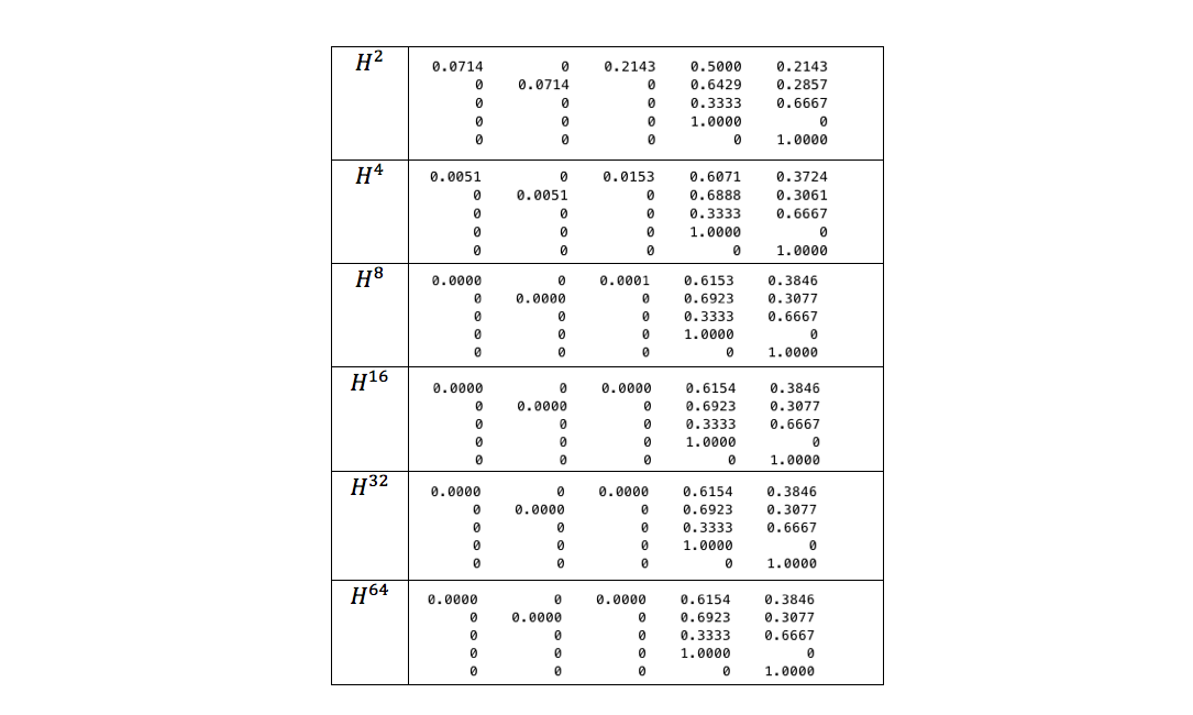
As can be seen from the table, already for

calculated probability

$H^8$

differs from the exact value that we previously obtained on the basis of the graph model, in 4 decimal places. Probability values calculated for

$P_{full}(c_1,CV)$

$H^{16}$ ,

$H^{32}$ ,

and do the same. Thus, in this case, it was enough to restrict ourselves to calculating

$H^{64}$

that requires everything

$H^8$

matrix multiplications. Thus, the rate of convergence of the limit to the required probability is rather high, which makes this model effective in practical applications.

$3$

From channel evaluation to optimization

The constructed analytical model allows to solve 3 main tasks:

Evaluate the effect of the channel on the conversion on the site
Rate the mutual influence of channels on each other
Estimate the likelihood that using a channel will result in a conversion on the site

When designing a conversion optimizer that allows you to manage your contextual advertising bids based on their performance so as to achieve the required

(key performance indicators) required to evaluate the conversion rate

$KPI$

for each key phrase. As we noted, the choice of a particular model of attribution of conversions directly affects the calculation of the conversion rate not only at the level of the advertising channel, but also at the level of the key phrase. Traditionally optimizers work with a model.

$CR$

or its modifications. We previously showed limited ability

$LCM$

predict the conversion rate (as a rule, it underestimates it, since it takes into account only the direct relationship of keyword conversion, without analyzing intermediate transitions). The presented model of attribution of conversions is free from these drawbacks, although it requires significantly more computational resources to calculate probabilities. The flexibility of the described approach also lies in the fact that we can use any integral attribute of the session as a “channel”. In particular, consider the parameter

$LCM$

, which was not used by us earlier in the calculations.

$URL$

contains information about the page on the site to which the user navigates at the beginning of the session. If the advertisement associated with the site is all marked up

$URL$

tagged, then we can significantly deepen our analytics.

$UTM-$

tagsare parameters (variables) containing additional data that are added to

$UTM$

target (landing) pages and allow you to transfer to the web analytics system additional information about the characteristics of traffic. Consider a typical example.

$URL$

tags, for example in the format adopted by the company

$UTM$

$Calltouch$ :

site.ru/?utm_source=YD&utm_medium=cpc&utm_content=kvartiry_ceny&utm_campaign=YD_KVARTIRY_POISK_MSK&calltouch_tm=yd_c :{campaign_id}_gb:{gbid}_ad:{ad_id}_ph:{phrase_id}_st:{source_type}_pt:{position_type}_p:{position}_s:{source}_dt:{device_type}_reg:{region_id}_ret:{retargeting_id}_apt:{addphrasestext}

Based on the dynamic parameters that are contained in curly brackets, we can, in particular, track the “path” of a click on an advertisement accurate to the key phrase that initiated the display of the advertisement that the user clicked on. We can choose any “reasonable” dynamic parameter (or a bunch of them) as a channel. In particular, if you select the parameter as a channel

$\ {phrase_ {id} \}$ , then we can track the user’s chain of transitions to the site using different keywords. If you repeat all the arguments for this type of channels, the model will allow you to calculate the total probability of conversion for each key phrase.

The resulting array of conversion factors can be used as input to the conversion optimizer.

Conclusion

This paper provides an overview of the currently used classical attribution attribution models. In addition, a multichannel attribution model based on Markov processes (chains) is described, which makes it possible to comprehensively evaluate both the probability of conversion for each advertising channel and calculate the effect of the channel on the conversion on the site. Demonstrated approaches to adapt the built model to optimize the rates in contextual advertising.

Source: https://habr.com/ru/post/343596/

All Articles

Multi-channel attribution through Calltouch

Introduction

Attribution models

Last Click Model

First Click Model

Linear model

Time decay

Position Type Model

How to choose an attribution model?

User sessions

Calculation of the influence of channels on the conversion

Estimate baseline metrics change when a channel is down

Model Description

Graph model

Matrix model

From channel evaluation to optimization

Conclusion

More articles: