Hi, Habr!

As they say, according to tradition, once a year we are rolling out something new at Yandex.Pododa. At first, it was Meteum - a traditional weather forecast using machine learning, then science - a short-term forecast of precipitation based on meteorological radars and neural networks. In this post, I will tell you about how we made a global weather forecast and built beautiful weather maps based on it.

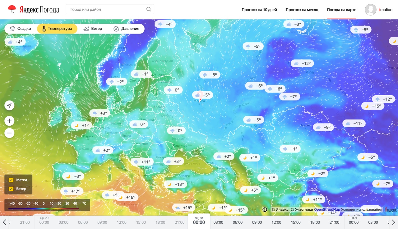
First a few words about the product. Weather maps - a way to find out the weather, which is very popular in the west and is not yet very popular in Russia. The reason for this is, in fact, the weather itself. Due to the climatic features, the most populated regions of our country are not subject to sudden weather disasters (and this is good). Therefore, the residents of these regions are more interested in the weather So, it is important for people in central Russia to know, for example, what kind of weather will be in Moscow at the weekend or that it will rain in St. Petersburg on Thursday. Such information is easiest to find out from the table, in which there will be a date, time and a set of weather parameters.

On the other hand, it is more important for residents of the US Eastern Coast to know the trajectory of the next hurricane with a beautiful female name, and for farmers from Dakota - to follow the spread of hail along the fields where corn is growing. Such information is much easier to learn from the map than from a variety of tables. So it turned out that weather services in Russia are rather tables, and in the West they are more like maps. However, in Russia there are patterns of weather consumption, when the user needs to know exactly where the weather will be, which he needs: these are people who choose a picnic place at the weekend, athletes, especially with the prefix "wind" and "kite" and, finally, summer residents . It is for these categories of users that we have made our product. And now I will talk about what is under his hood.

Forecast calculation: personal and global

We immediately decided that in order to build maps, our forecast should become global. Well, if only because the maps covering not the entire globe, give the Middle Ages. Thus, we needed to expand Meteum to global coverage. However, the previous system architecture was not very scalable.

Summary of the previous series. As the attentive reader remembers, in the first implementation of Meteum we calculated the weather forecast as necessary. As soon as the user got to our site, we collected a list of factors for his coordinates and transferred to the trained MatrixNet model. Microservice was responsible for collecting factors, which we called vector-api. Microservice was good for all but one: when adding new factors and / or expanding the geography of coverage, we were approaching the memory limit of the physical machines on which microservice worked. In addition, in itself, the formation of the response of the final weather API contained a time-consuming and processor-intensive operation using the Matriksnet model. Both factors strongly impeded the construction of a global forecast. Plus, in our backlog, there was a whole line of factors that increased the accuracy of the prediction in the experiments, but could not go into production due to the limitations described above.

We also faced the shortcomings of the chosen architecture for the precipitation map, hotly beloved by many users. For the storage and processing of data necessary for the construction of precipitation information, PostgreSQL DBMS with the PostGIS extension was used. During summer thunderstorms, the number of requests to heavy handles per second lightning-fast turned from hundreds to tens of thousands, which entailed a high consumption of processors and network channels of database servers. These circumstances served as an additional incentive to think about the future of the service and apply a different approach in processing and storing weather data.

An alternative to calculating the weather in runtime was a preliminary calculation of forecasts for a large set of coordinates as the factors were updated. We settled on a global grid covering land with a resolution of 2x2 km, and water with a resolution of 10x10 km. The grid is divided into squares of 3 to 3 degrees - these squares allow us to simultaneously prepare factors for the model and process the results. Here is how it looks on the map.

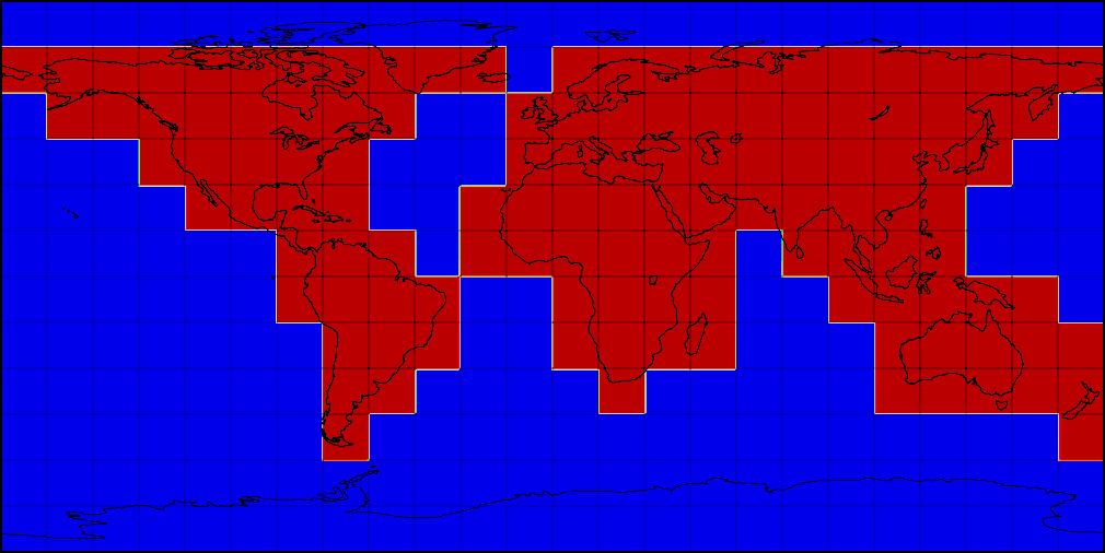
Splitting global regular grid areas

The process of preparing weather factors begins with the Meteo cluster. According to the name, “classical meteorology” takes place on this cluster. Here we download observational data and forecasts of GFS (USA), ECMWF (England), JMA (Japan), CMC (Canada), EUMETSAT (France), Earth Networks (USA) and many other suppliers. Here is the calculation of the weather model WRF for the most interesting regions for us. Meteorological data obtained from partners or as a result of calculations is usually packed in GRIB or NetCDF formats with different levels of compression. Depending on the supplier or method of calculation, this data may cover the Moscow region or the whole world and weigh from 200MB to 7GB.

From a meteocluster, the weather forecast files first go to MDS (Media Storage, storage for large pieces of binary information), and then to YT - our Yandex Map-Reduce system. Work in YT is divided into two stages, conditionally called "supply" and "application." Supply is the preparation of factors for the subsequent application of a trained model. Factors should be correctly re-interpolated to the final grid, lead to a single unit of measurement and cut into 3 by 3 degrees squares for parallel processing and application. The complexity of the procedure here lies in the large amounts of data and the need to do an exercise every time a new forecast data has arrived for a particular area.

After the first step has worked, the application of pre-trained machine learning models begins. In the first implementation of Meteum, we could predict only two main weather parameters using machine learning: temperature and precipitation. Now that we have switched to a new calculation scheme, we can use the same approach to calculate the remaining weather parameters. The use of machine learning gives a tangible increase in accuracy for new parameters: pressure, wind speed and humidity. The forecast error of these parameters for 24 hours ahead drops by up to 40%. In addition to the fact that for many users, the most accurate wind and pressure indicators are important, this improvement allows us to more accurately calculate another popular parameter - temperature on sensations. It consists of normal temperature, wind speed and humidity. Another notable innovation was the new method of calculating weather phenomena. Now it is based on a multi-classification formula - it determines not only the presence or absence of precipitation, but also their type (rain, snow, hail), and the presence and intensity of cloudiness.

All these models need to be applied for a limited time for each point of the regular grid. After the models have been applied, there is another layer of data processing - business logic. In this section, we bring the variables predicted by machine learning to the units we need, and also make the forecast consistent. Since right now the ML models know little enough about the physics of processes, mainly relying on factors derived from meteorological models, we can get inconsistent weather conditions, such as "rain at a temperature of -10". We have ideas on how to do more correctly in this place, but right now this is being solved by formal constraints.

The difficulty in applying the trained models is that for each prediction, it is necessary to perform about 14 billion operations. There are hundreds of factors necessary for each calculation, and the list of these factors is very mobile: we constantly experiment with them, try new ones, add whole groups, throw out weak ones. Not all factors are taken directly from suppliers. We are experimenting with factor-functions of several parameters. The rules for forming such a number of features are very difficult to maintain as a Python code: it is cumbersome, it is difficult to do lazy calculations, it is difficult to analyze and diagnose which features (or source data for features) are no longer needed. Therefore, we invented its own analogue LISP. Strictly speaking, this is not a LISP, but a ready-made AST, which is very similar to the LISP dialect, which takes into account the specificity of our data. We made the processor of this LISP the way we need it: lazy and caching. Therefore, we, firstly, do not calculate factors that are no longer needed, and secondly, do not calculate twice what we need twice. These mechanisms automatically apply to all calculations. And thanks to the fact that this is a formal AST, we can: easily analyze what is needed and what is not needed; serialize and store separate parts of logic, write business parts into logs, form large parts of logic automatically (bypassing the presentation in the form of code), version them for experiments, and so on. The overhead turned out to be completely insignificant, since all operations are performed immediately above the matrices.

The general scheme of data delivery to the API

After calculating the forecasts, we write them into a special format - ForecastContainer and load these containers into the microservice to return data from the memory. The fact is that for the whole world with our grid of 0.02 degrees we get about 1 166 400 000 floating point values, and this is 34 GB of data for only one parameter. We have more than 50 such parameters - therefore, it was not possible to keep this data completely in the memory of one physical machine. We began to look for a format that supports fast reading of compressed data. The first candidate was HDF5 - which has the functionality of chunking data and buffer support for unpacked chunks. The second candidate was our self-proprietary format — the matrices of floats compressed by LZ4 and recorded in Flatbuffer. The test results showed that opening a file with data for work takes two times less time for Flatbuffers than for HDF5, as well as reading an arbitrary point from the cache. As a result, now the data for 50 variables occupy 52.1GB.

Since the requirements for memory consumption and response time were very high since the formulation of the problem, we decided to rewrite the old microservice written in Python in C ++. And it gave its results: The response time of the service in 99 quantile fell from 100ms to 10ms.

The transfer of the service to the new backend architecture allowed us to give weather forecasts to our internal and external partners directly, bypassing the caches and model calculations in runtime, made it possible, with an urgent need, to easily scale the load using Yandex cloud technologies.

In total, the new architecture allowed us to reduce the response timings, keep a lot of work and get rid of the data that was given to different partners. Yandex.Pogoda data is represented in a large number of Yandex services and not only: the Yandex main page, the weather plugin in Yandex. Browser, the weather on the Rambler, and so on. As a result, they all had the opportunity to give exactly the values ​​that the users of the main Yandex.Pogoda page see at that moment.

Closer to the people: Tile server and front

In order to draw forecasts on our new maps, a lot of additional processing is needed. First, we run MapReduce operations on the same data that is given by microservice and API to generate data for the whole world on a regular latitudinal-longitudinal grid with a resolution of 0.02 degrees. At the output for each parameter: temperature, pressure, wind speed and direction, as well as for each horizon: forecast time in the future or fact time in the past, we get the matrix of size 9001 * 18000.

After that, we build the Mercator projection using this data and cut them into tiles in accordance with the requirements of the Yandex.Maps API. Here we meet with one of the biggest difficulties in the chain of preparing weather maps: the number of tiles that need to be updated promptly when generating each new forecast. So, each next level of map zooming requires 4 times more tiles than the previous one. It is easy to estimate that for all levels of approximation from 0 up to 8 you need to prepare

$$

$$4 ^ 0 + 4 ^ 1 + \ dots + 4 ^ 7 = $ 2184$$

pictures. In total, for each of the four parameters, we show 25 horizons, of which there are 12 forecasts for the future. Therefore, every hour it is required to update 1048560 pictures.

As the pictures are ready, we upload them to the internal storage of Yandex files with high parallelism. As soon as the entire map layer for all the zooms is loaded, we replace the index value, according to which the front understands where to go for the new tiles. Thus, a sufficiently high rate of appearance of new forecasts on the map and consistency of data within the forecast time is achieved.

Even despite the serious preparation on the back end, drawing and animating weather maps is also a difficult task. It’s impossible to tell everything in one article, so here we have focused on the most noticeable feature - the rendering of animated particles, showing the direction of wiping.

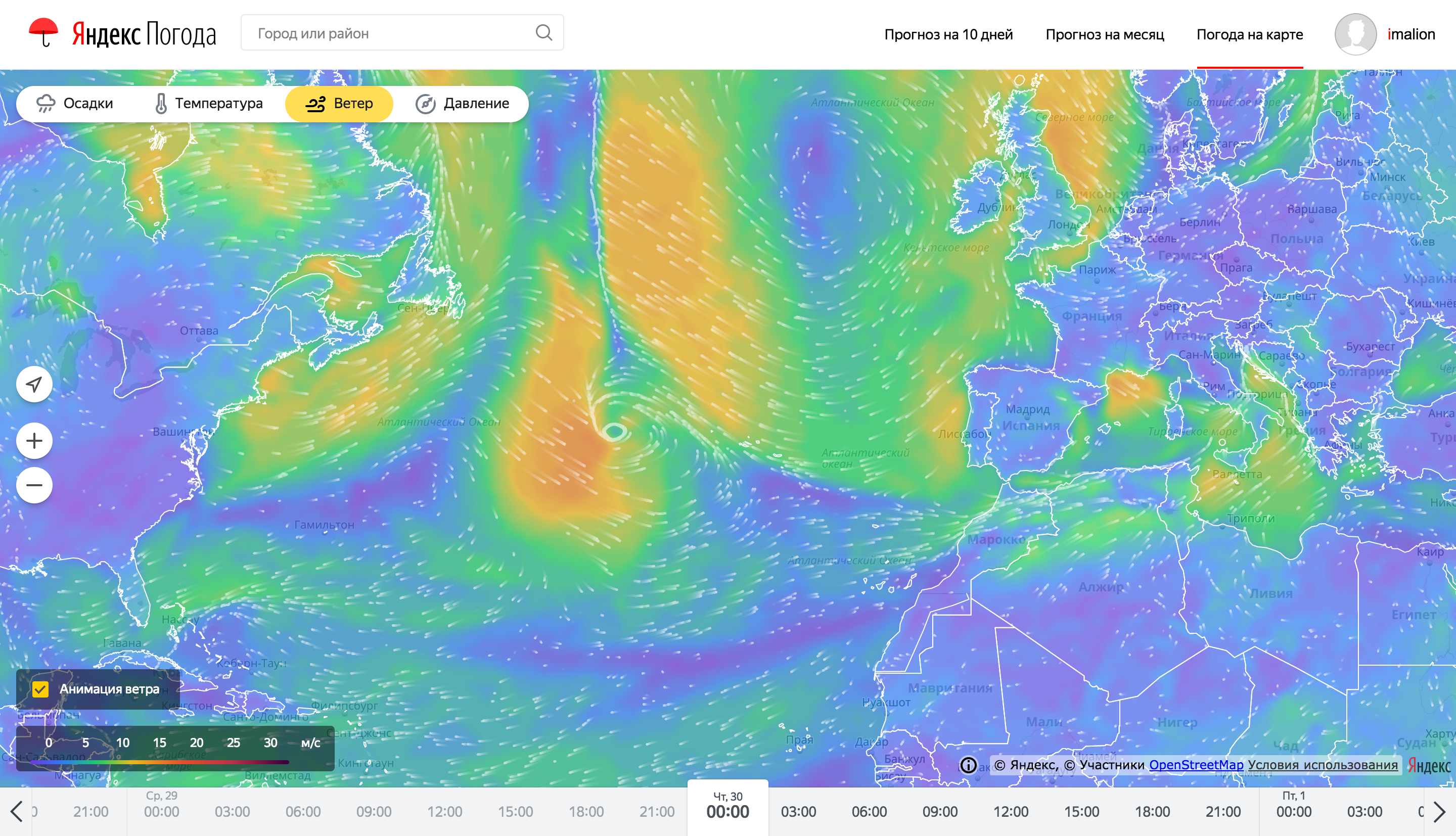
This is how the wind animation particles look on weather maps.

To optimize the resource consumption of the client device, wind animation was performed using WebGL. WebGL allows you to use significant graphics adapter resources, offloading the processor's flow of code execution, as well as optimizing battery consumption. The task of the processor in this case is to set the execution arguments for shader programs. To move the particles, the particle position storage approach is used in 2x texture color channels for each axis (x / y). There are two such textures of position: one stores the current position of the particles, the second is designed to preserve the new state.

The process of particle rendering is described by several WebGL programs. For greater compatibility, the first version of this standard is used. In a browser, using WebGL is done through the corresponding context of the canvas element. Since the graphics accelerator is capable of performing several times more parallel operations through a processor, the movement of particles should be performed through the WebGL program. The output of such a program is a set of points in a given space. This default space is the visible area of ​​your canvas, that is, the user's screen. However, it is possible to specify the purpose of rendering the texture using framebuffers.

When the wind layer starts, the processor generates the initial position of the particles, creating a typed array of elements in the range of 0 ... 255, in an amount (particles * components) (RGBA). From this array, two WebGL location textures are created. Data on wind speed is also recorded in the texture so that the video card has access to them. The red and green channels of this texture contain the value of parallel and meridional speeds, respectively, where the value 127 corresponds to the absence of wind, values ​​less than 127 set the wind speed in the negative direction along the axis, the values ​​more - in positive. Using the prepared textures, the current position of the particles is drawn. After rendering, one of the position textures is updated using the second texture as the source of the current state data. The following visible frames will be formed by drawing the previous image of the position of the particles with increased transparency, on top of which the current position of the particles will be plotted. Thus particles with damped tails are obtained.

This is how the particles of the wind animation look like in the process of their creation.

As it turned out, the current algorithm for coding the position of particles in texture pixels for high-quality visualization requires support at the hardware level of high precision calculations and float values ​​in the textures themselves, which is often not the case on mobile devices, so the algorithm will be revised and improved.

Conclusion and plans

Here's about everything that I wanted to tell you about the architecture of Yandex. Weather. During this year, we completely redesigned the service from the inside (described above) and outside (almost all the platforms on which Ya.Pogoda is present were significantly redrawn). The final of these changes were interactive weather maps that you can try on our service .

However, we never rest on our laurels. Next year you will find a lot of interesting grocery and technological updates: from the service that allows you to explore the climate in different parts of the Earth to the answer to the question "what does a person breathe". And this, of course, not all. Stay with us.

Always yours,
Team Yandex.Pogody