Quantum versus classical: why do we need so many digits
Because of the general boom of the blockchain and every bigdata, another promising topic came down from the first lines of technical news - quantum computing. And they, by the way, are able to turn several IT areas at once, starting with the notorious blockchain and ending with information security. In the next two articles, Sberbank and Sberbank-Technologies will tell you what quantum computations are cool with and what they generally do with them now.

To deal with quantum computing, it is worth to begin to refresh the knowledge of classical ones. Here the unit of information processed is the bit. Each bit can only be in one of two possible states - 0 or 1. A register of N bits can contain one of 2 N possible combinations of states and is represented as their sequence.
To process and transform information, bitwise operations from Boolean algebra are used. Basic operations are single-bit NOT and double-bit AND and OR. Bit operations are described through truth tables. They match the input arguments with the resulting value.
')
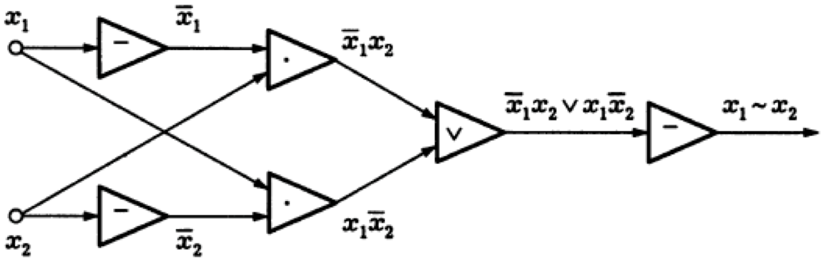
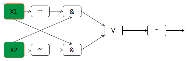
The algorithm of classical calculations is a set of consecutive bit operations. It is most convenient to reproduce it graphically, in the form of a diagram of functional elements (SFE), where each operation has its own designation. Here is an example of an SFE to test two bits for equivalence.
Now let's move on to a new topic. Quantum computing is an alternative to classical algorithms based on the processes of quantum physics. It says that without interaction with other particles (that is, until the time of measurement), the electron does not have unambiguous coordinates on the orbit of the atom, but is simultaneously located in all points of the orbit. The region in which the electron is located is called the electron cloud. In a known experiment with two slits, one electron passes simultaneously through both slits, interfering with itself. Only when measuring this uncertainty collapses and the coordinates of the electron become unambiguous.

The probabilistic nature of measurements inherent in quantum computation underlies many algorithms — for example, searching in an unstructured database. Algorithms of this type incrementally increase the amplitude of the correct result, allowing you to get it at the output with the maximum probability.
In quantum computing, the physical properties of quantum objects are implemented in the so-called qubits (q-bit). A classic bit can only be in one state - 0 or 1. A qubit before measurement can be in both states at the same time; therefore, it is usually denoted by the expression a | 0⟩ + b | 1⟩, where A and B are complex numbers that satisfy the condition | A | 2 + | B | 2 = 1. The measurement of a qubit instantly “collapses” its state into one of the basic ones, 0 or 1. At the same time, the “cloud” collapses into a point, the initial state is destroyed, and all information about it is irretrievably lost.
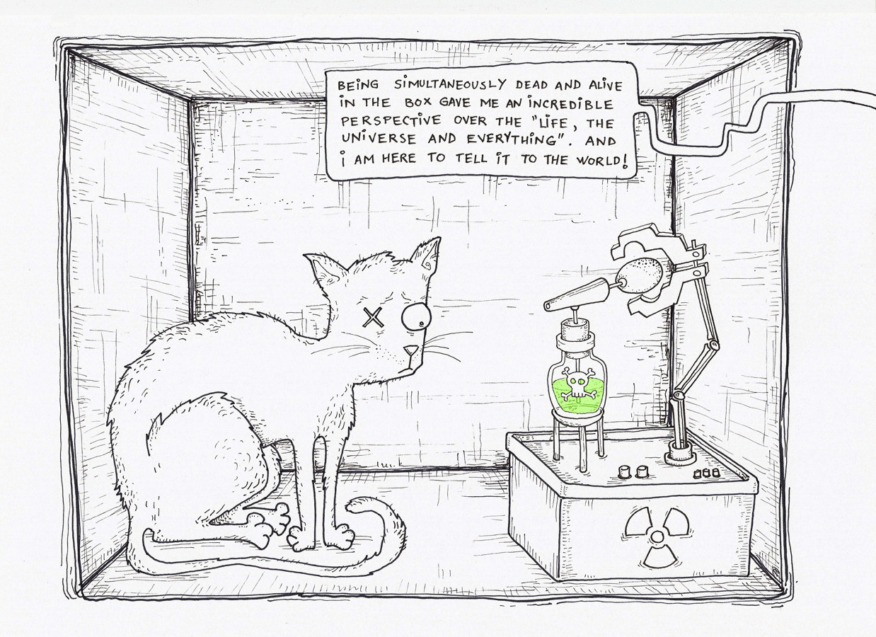
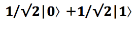
One of the uses of this property isSchrödinger's cat, a generator of truly random numbers. A qubit is entered into a state in which the result of measurement can be 1 or 0 with the same probability. This state is described as:
Let's start with the basics. There is a set of input data for calculations, represented in binary format by vectors of length N.
In classical calculations, only one of the 2n data options is loaded into the computer's memory, and the function value is calculated for this variant. As a result, only one of the 2 n possible data sets is processed simultaneously.
All 2 n combinations of the initial data are simultaneously presented in the memory of a quantum computer. Conversions are applied to all of these combinations at once. As a result, in one operation, we calculate the function for all 2 n possible variants of the data set (the measurement will eventually only give one solution, but more on that later).
Both classical and quantum computing use logical transformations - gates . In classical calculations, the input and output values are stored in different bits, which means that the number of inputs in gates can differ from the number of outputs:

Consider the real problem. It is necessary to determine whether two bits are equivalent.
If in classical calculations at the output we get one, then they are equivalent, otherwise there isn’t:
Now imagine this problem using quantum computing. In them, all conversion gates have as many outputs as inputs. This is due to the fact that the result of the transformation is not a new value, but a change in the state of the current.
In the example, we compare the values of the first and second qubits. The result will be in the zero qubit - the qubit-flag. This algorithm is applicable only to the base states - 0 or 1. Here is the order of quantum transformations.
Let's try to compare classical and quantum calculations in more serious problems. For this we need a little more theoretical knowledge.
In quantum computing, the processed information is encoded in quantum bits, the so-called qubits. In the simplest case, a qubit, like the classic bit, can be in one of two basic states: | 0⟩ (a short designation for the vector 1 | 0⟩ + 0 | 1⟩) and | 1⟩ (for the vector 0 | 0⟩ + 1 | 1⟩). The quantum register is a tensor product of the qubit vectors. In the simplest case, when each qubit is in one of the basic states, the quantum register is equivalent to the classical one. The register of two qubits in the state | 0> can be described as follows:
(1 | 0⟩ + 0 | 1⟩) * (1 | 0⟩ + 0 | 1⟩) = 1 | 00⟩ + 0 | 01⟩ + 0 | 10⟩ + 0 | 11⟩ = | 00⟩.
For processing and transforming information in quantum algorithms, so-called quantum gates (gates) are used. They are represented as a matrix. To obtain the result of applying the gate, we need to multiply the vector characterizing the qubit by the gate's matrix. The first coordinate of the vector is the factor in front of | 0, the second coordinate is the factor in front of | 1⟩. The matrix of basic single-qubit gates looks like this:

Here is an example of using the gate Not:
X * | 0⟩ = X * (1 | 0⟩ + 0 | 1⟩) = 0 | 0⟩ + 1 | 1⟩ = | 1⟩
The multipliers before the base states are called amplitudes and are complex numbers. The modulus of a complex number is equal to the root of the sum of the squares of the real and imaginary parts. The square of the amplitude module facing the baseline state is equal to the probability of obtaining this baseline state when measuring the qubit, therefore the sum of squares of the amplitude modules is always 1. We could use arbitrary matrices for transformations over qubits, but due to the fact that the norm (length) vectors should always be equal to 1 (the sum of the probabilities of all outcomes is always 1), our transformation must preserve the norm of the vector. So the transformation must be unitary and the corresponding matrix is unitary. Recall that the unitary transformation is reversible and UU † = I.
For more visual work with qubits, they are represented by vectors on the Bloch sphere. In this interpretation, single-qubit gates represent the rotation of the qubit vector around one of the axes. For example, the gate Not (X) rotates the qubit vector on Pi relative to the X axis. Thus, the state | 0>, represented by a vector directed strictly upwards, changes to the state | 1>, directed strictly downwards. The state of a qubit on the Bloch sphere is defined by the formula cos (θ / 2) | 0⟩ + e iϕ sin (θ / 2) | 1⟩
To build algorithms, it is not enough for us to have single-qubit gates. Gates are needed that carry out transformations depending on certain conditions. The main such tool is the two-qubit gate CNOT. This gate is applied to two qubits and inverts the second qubit only if the first qubit is in the | 1⟩ state. The CNOT gate matrix looks like this:
Here is an example of application:
CNOT * | 10⟩ = CNOT * (0 | 00⟩ + 0 | 01⟩ + 1 | 10⟩ + 0 | 11⟩) = 0 | 00⟩ + 0 | 01⟩ + 1 | 11⟩ + 0 | 10⟩ = | 11⟩
Using the CNOT gate is equivalent to performing the classic XOR operation with writing the result to the second qubit. Indeed, if you look at the truth table of the operator XOR and CNOT, you will see a match:
The gate of CNOT has an interesting property - after its application, qubits are entangled or unraveled, depending on the initial state. This will be shown in the next article, in the section on quantum parallelism.
Having a full arsenal of quantum gates, we can begin to develop quantum algorithms. In the graphical representation, qubits are represented by straight lines - “strings”, on which gates overlap. The single qubit Pauli gates are denoted by the usual squares inside which the axis of rotation is depicted. Gate CNOT looks a bit more complicated:
An example of the application of the gate CNOT:
One of the most important actions in the algorithm is to measure the result. Measurement is usually indicated by an arc scale with an arrow and the designation of which axis is being measured.
So, let's try to build a classical and quantum algorithm, which adds 3 to the argument.
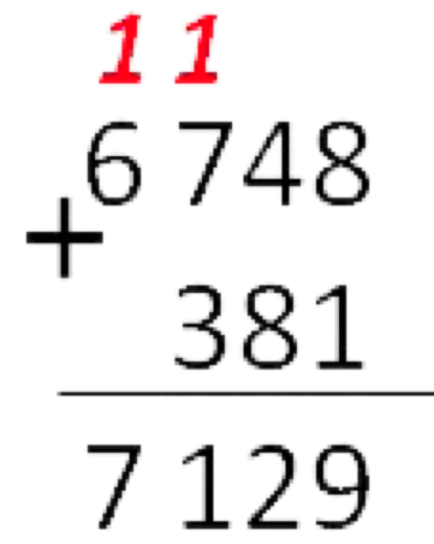
Summing ordinary numbers with a bar implies performing two actions on each digit — the sum of the digits themselves and the sum of the result with the transfer from the previous operation, if such transfer was.
In the binary representation of numbers, the summation operation will consist of the same actions. Here is the python code:
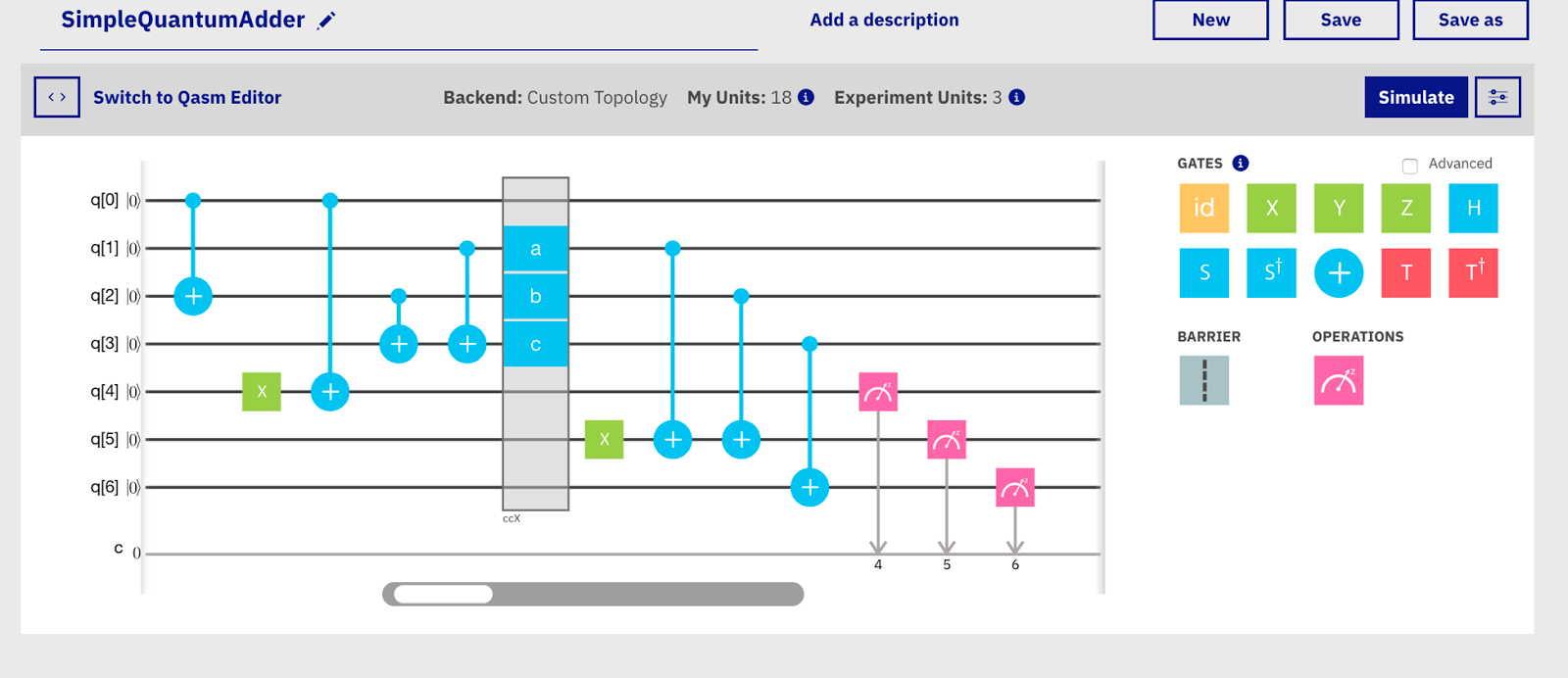
Now let's try to develop a similar program for a quantum calculator:

In this scheme, the first two qubits are the argument, the next two are hyphens, the remaining 3 are the result. This is how the algorithm works.
By running both examples, we get the same result. On a quantum computer, this will take more time, because it is necessary to conduct an additional compilation into a quantum-assembler code and send it to execution to the cloud. The use of quantum computing would make sense if the speed of performing their elementary operations — gates — would be many times less than in the classical model.
Measurements of experts show that the execution of one gate takes about 1 nanosecond. So the algorithms for a quantum computer must not copy the classical ones, but rather use the unique properties of quantum mechanics to the maximum. In the next article we will examine one of the main such properties - quantum parallelism - and talk about quantum optimization in general. Then we determine the most appropriate areas for quantum computing and discuss their application.
Based on materials by Dmitry Sapayev , senior director of IT development in the development department of Sberbank Technologies, and Dmitry Bulychkov, project director at the Center for Technological Innovations of Sberbank.
UPD : We published the second part of the article , where we dive into quantum computations more deeply and talk about their practical application.
Classical calculations: AND, OR, NOT
To deal with quantum computing, it is worth to begin to refresh the knowledge of classical ones. Here the unit of information processed is the bit. Each bit can only be in one of two possible states - 0 or 1. A register of N bits can contain one of 2 N possible combinations of states and is represented as their sequence.
To process and transform information, bitwise operations from Boolean algebra are used. Basic operations are single-bit NOT and double-bit AND and OR. Bit operations are described through truth tables. They match the input arguments with the resulting value.
')
The algorithm of classical calculations is a set of consecutive bit operations. It is most convenient to reproduce it graphically, in the form of a diagram of functional elements (SFE), where each operation has its own designation. Here is an example of an SFE to test two bits for equivalence.
Quantum computing Physical basis
Now let's move on to a new topic. Quantum computing is an alternative to classical algorithms based on the processes of quantum physics. It says that without interaction with other particles (that is, until the time of measurement), the electron does not have unambiguous coordinates on the orbit of the atom, but is simultaneously located in all points of the orbit. The region in which the electron is located is called the electron cloud. In a known experiment with two slits, one electron passes simultaneously through both slits, interfering with itself. Only when measuring this uncertainty collapses and the coordinates of the electron become unambiguous.
The probabilistic nature of measurements inherent in quantum computation underlies many algorithms — for example, searching in an unstructured database. Algorithms of this type incrementally increase the amplitude of the correct result, allowing you to get it at the output with the maximum probability.
Qubits
In quantum computing, the physical properties of quantum objects are implemented in the so-called qubits (q-bit). A classic bit can only be in one state - 0 or 1. A qubit before measurement can be in both states at the same time; therefore, it is usually denoted by the expression a | 0⟩ + b | 1⟩, where A and B are complex numbers that satisfy the condition | A | 2 + | B | 2 = 1. The measurement of a qubit instantly “collapses” its state into one of the basic ones, 0 or 1. At the same time, the “cloud” collapses into a point, the initial state is destroyed, and all information about it is irretrievably lost.
One of the uses of this property is
Quantum and classical calculations. First round
Let's start with the basics. There is a set of input data for calculations, represented in binary format by vectors of length N.
In classical calculations, only one of the 2n data options is loaded into the computer's memory, and the function value is calculated for this variant. As a result, only one of the 2 n possible data sets is processed simultaneously.
All 2 n combinations of the initial data are simultaneously presented in the memory of a quantum computer. Conversions are applied to all of these combinations at once. As a result, in one operation, we calculate the function for all 2 n possible variants of the data set (the measurement will eventually only give one solution, but more on that later).
Both classical and quantum computing use logical transformations - gates . In classical calculations, the input and output values are stored in different bits, which means that the number of inputs in gates can differ from the number of outputs:
Consider the real problem. It is necessary to determine whether two bits are equivalent.
If in classical calculations at the output we get one, then they are equivalent, otherwise there isn’t:
Now imagine this problem using quantum computing. In them, all conversion gates have as many outputs as inputs. This is due to the fact that the result of the transformation is not a new value, but a change in the state of the current.
In the example, we compare the values of the first and second qubits. The result will be in the zero qubit - the qubit-flag. This algorithm is applicable only to the base states - 0 or 1. Here is the order of quantum transformations.
- We act on the qubit-flag with the “He” gate, exposing it to 1.
- Two times we use the two-bit gate “Controlled Not”. This gate changes the value of the qubit flag to the opposite only if the second qubit involved in the transformation is in state 1.
- We measure the zero qubit. If the result is 1, then both the first and second qubits are either both in state 1 (the qubit-flag has changed its value twice), or in state 0 (the qubit-flag has remained in state 1). Otherwise, qubits are in different states.
Next level. Quantum single qubit gates of Pauli
Let's try to compare classical and quantum calculations in more serious problems. For this we need a little more theoretical knowledge.
In quantum computing, the processed information is encoded in quantum bits, the so-called qubits. In the simplest case, a qubit, like the classic bit, can be in one of two basic states: | 0⟩ (a short designation for the vector 1 | 0⟩ + 0 | 1⟩) and | 1⟩ (for the vector 0 | 0⟩ + 1 | 1⟩). The quantum register is a tensor product of the qubit vectors. In the simplest case, when each qubit is in one of the basic states, the quantum register is equivalent to the classical one. The register of two qubits in the state | 0> can be described as follows:
(1 | 0⟩ + 0 | 1⟩) * (1 | 0⟩ + 0 | 1⟩) = 1 | 00⟩ + 0 | 01⟩ + 0 | 10⟩ + 0 | 11⟩ = | 00⟩.
For processing and transforming information in quantum algorithms, so-called quantum gates (gates) are used. They are represented as a matrix. To obtain the result of applying the gate, we need to multiply the vector characterizing the qubit by the gate's matrix. The first coordinate of the vector is the factor in front of | 0, the second coordinate is the factor in front of | 1⟩. The matrix of basic single-qubit gates looks like this:
Here is an example of using the gate Not:
X * | 0⟩ = X * (1 | 0⟩ + 0 | 1⟩) = 0 | 0⟩ + 1 | 1⟩ = | 1⟩
The multipliers before the base states are called amplitudes and are complex numbers. The modulus of a complex number is equal to the root of the sum of the squares of the real and imaginary parts. The square of the amplitude module facing the baseline state is equal to the probability of obtaining this baseline state when measuring the qubit, therefore the sum of squares of the amplitude modules is always 1. We could use arbitrary matrices for transformations over qubits, but due to the fact that the norm (length) vectors should always be equal to 1 (the sum of the probabilities of all outcomes is always 1), our transformation must preserve the norm of the vector. So the transformation must be unitary and the corresponding matrix is unitary. Recall that the unitary transformation is reversible and UU † = I.
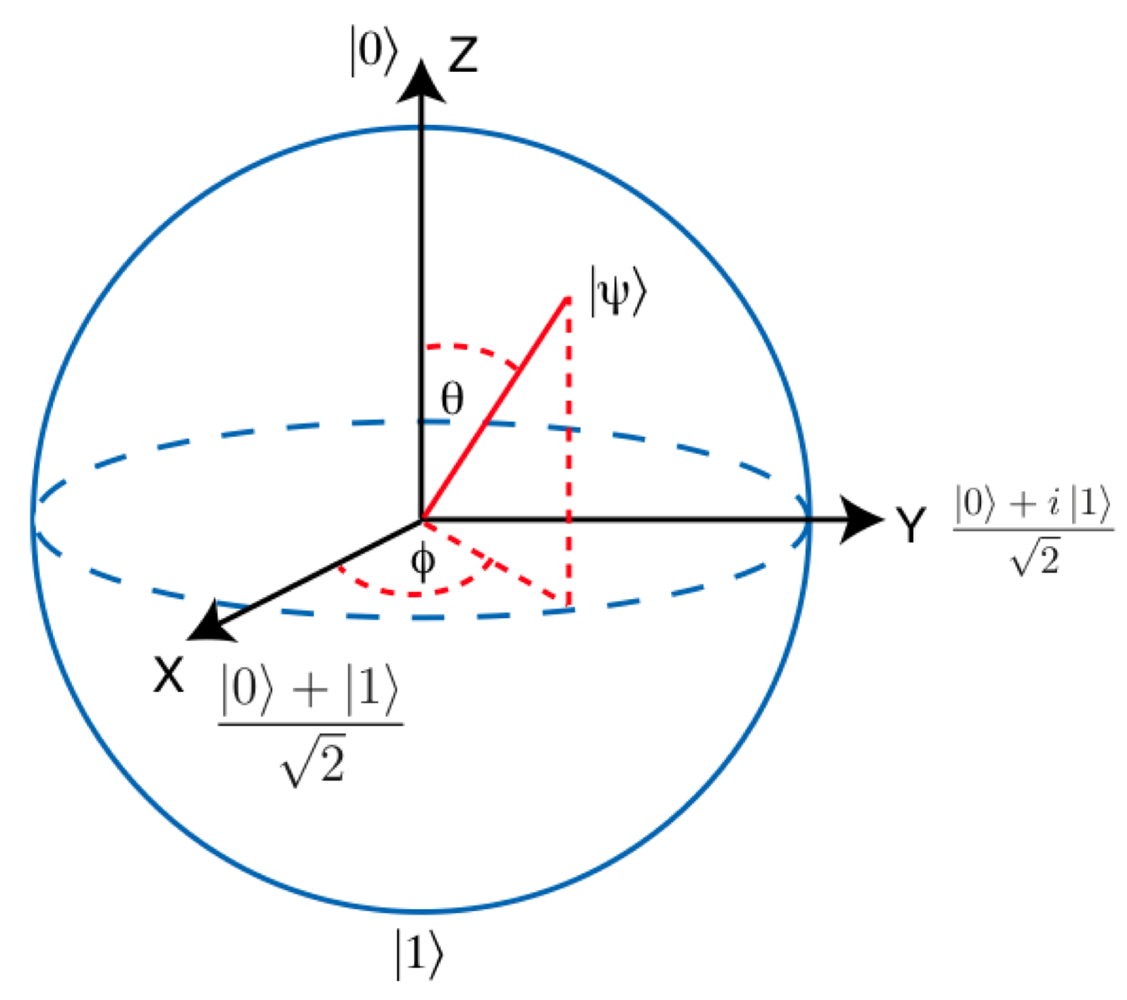
For more visual work with qubits, they are represented by vectors on the Bloch sphere. In this interpretation, single-qubit gates represent the rotation of the qubit vector around one of the axes. For example, the gate Not (X) rotates the qubit vector on Pi relative to the X axis. Thus, the state | 0>, represented by a vector directed strictly upwards, changes to the state | 1>, directed strictly downwards. The state of a qubit on the Bloch sphere is defined by the formula cos (θ / 2) | 0⟩ + e iϕ sin (θ / 2) | 1⟩
Quantum two-qubit gates
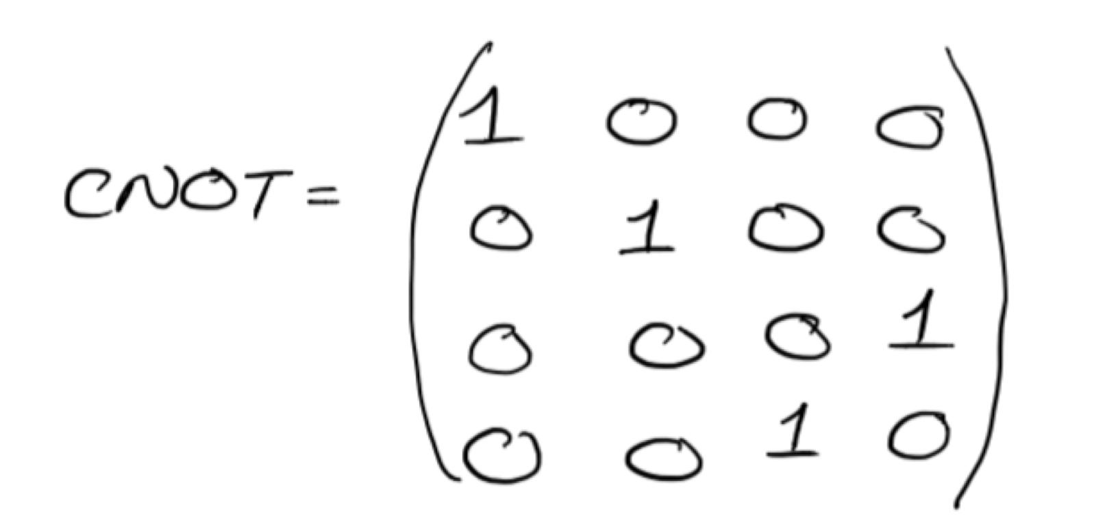
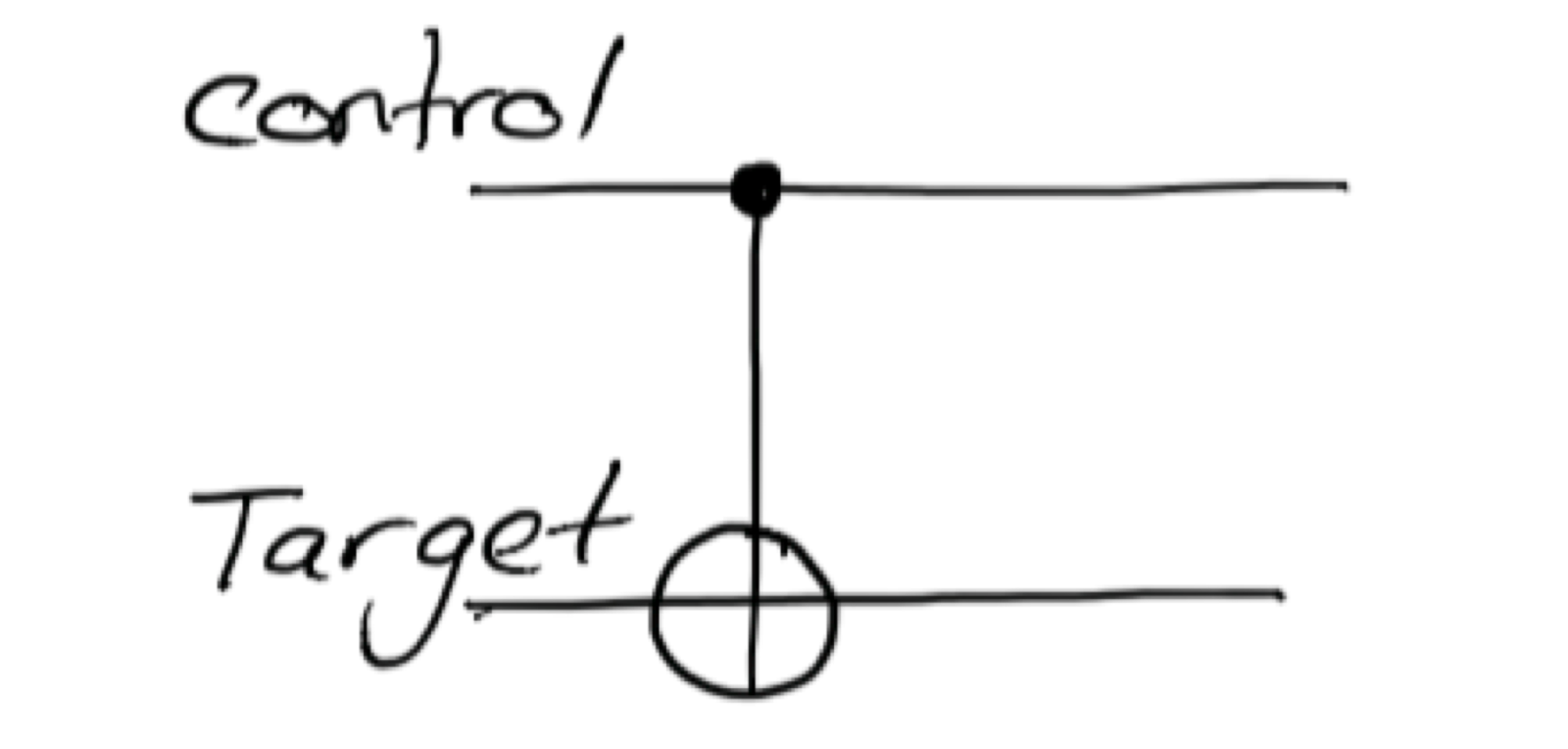
To build algorithms, it is not enough for us to have single-qubit gates. Gates are needed that carry out transformations depending on certain conditions. The main such tool is the two-qubit gate CNOT. This gate is applied to two qubits and inverts the second qubit only if the first qubit is in the | 1⟩ state. The CNOT gate matrix looks like this:
Here is an example of application:
CNOT * | 10⟩ = CNOT * (0 | 00⟩ + 0 | 01⟩ + 1 | 10⟩ + 0 | 11⟩) = 0 | 00⟩ + 0 | 01⟩ + 1 | 11⟩ + 0 | 10⟩ = | 11⟩
Using the CNOT gate is equivalent to performing the classic XOR operation with writing the result to the second qubit. Indeed, if you look at the truth table of the operator XOR and CNOT, you will see a match:
| XOR | CNOT | |||
| 0 | 0 | 0 | 00 | 00 |
| 0 | one | one | 01 | 01 |
| one | 0 | one | ten | eleven |
| one | one | 0 | eleven | ten |
The gate of CNOT has an interesting property - after its application, qubits are entangled or unraveled, depending on the initial state. This will be shown in the next article, in the section on quantum parallelism.
Algorithm construction - classical and quantum implementation
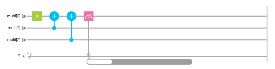
Having a full arsenal of quantum gates, we can begin to develop quantum algorithms. In the graphical representation, qubits are represented by straight lines - “strings”, on which gates overlap. The single qubit Pauli gates are denoted by the usual squares inside which the axis of rotation is depicted. Gate CNOT looks a bit more complicated:
An example of the application of the gate CNOT:
One of the most important actions in the algorithm is to measure the result. Measurement is usually indicated by an arc scale with an arrow and the designation of which axis is being measured.
So, let's try to build a classical and quantum algorithm, which adds 3 to the argument.
Summing ordinary numbers with a bar implies performing two actions on each digit — the sum of the digits themselves and the sum of the result with the transfer from the previous operation, if such transfer was.
In the binary representation of numbers, the summation operation will consist of the same actions. Here is the python code:
arg = [1,1] # result = [0,0,0] # carry1 = arg[1] & 0x1 # 0b11, , = 1 result[2] = arg[1] ^ 0x1 # carry2 = carry1 | arg[0] # 0b11, , = 1 result[1] = arg[0] ^ 0x1 # result[1] ^= carry1 # result[0] ^= carry2 # print(result) Now let's try to develop a similar program for a quantum calculator:
In this scheme, the first two qubits are the argument, the next two are hyphens, the remaining 3 are the result. This is how the algorithm works.
- The first step before the barrier we put the argument in the same state as in the classic case - 0b11.
- Using the CNOT operator, we calculate the value of the first transfer — the result of the operation arg & 1 is equal to one only when arg is 1, in this case we invert the second qubit.
- The next 2 gates implement addition of the lower bits - we transfer the qubit 4 to the state | 1⟩ and write the XOR result to it.
- The large rectangle indicates the gate CCNOT, an extension of the CNOT gate. In this gate, there are two control qubits and the third is inverted only if the first two are in the | 1 state. The combination of 2 gate CNOT and one CCNOT gives us the result of the classic operation carry2 = carry1 | arg [0]. The first 2 gates set a carry to unit if one of them is equal to 1, and the CCNOT gate handles the case when they both are equal to one.
- We add higher qubits and carry qubits.
Intermediate conclusions
By running both examples, we get the same result. On a quantum computer, this will take more time, because it is necessary to conduct an additional compilation into a quantum-assembler code and send it to execution to the cloud. The use of quantum computing would make sense if the speed of performing their elementary operations — gates — would be many times less than in the classical model.
Measurements of experts show that the execution of one gate takes about 1 nanosecond. So the algorithms for a quantum computer must not copy the classical ones, but rather use the unique properties of quantum mechanics to the maximum. In the next article we will examine one of the main such properties - quantum parallelism - and talk about quantum optimization in general. Then we determine the most appropriate areas for quantum computing and discuss their application.
Based on materials by Dmitry Sapayev , senior director of IT development in the development department of Sberbank Technologies, and Dmitry Bulychkov, project director at the Center for Technological Innovations of Sberbank.
UPD : We published the second part of the article , where we dive into quantum computations more deeply and talk about their practical application.
Source: https://habr.com/ru/post/343308/
All Articles