Binary Matrix Neural Network
An artificial neural network in the form of a matrix, the inputs and outputs of which are sets of bits, and the neurons implement the functions of the binary logic of several variables. Such a network is significantly different from perceptron type networks and can provide such advantages as a finite number of options for a complete exhaustive search of network functions, and therefore a finite learning time, and the relative simplicity of hardware implementation.

Attempts to create artificial neural networks are based on the fact of the existence of their natural prototypes. The method of transmitting and processing information in the natural neural network is determined by the chemical and biological properties of living neuron cells. However, the model of an artificial neural network does not have to completely copy both the function of the neurons and the structure of the natural brain, since it implements only the function of transforming information inputs into the outputs. Therefore, the implementation of the function of an artificial neural network may differ significantly from its natural counterpart. An attempt to directly copy the structure of the natural brain inevitably encounters the following problems, which, in the absence of their solution, may prove to be insurmountable. As you know, in the mammalian brain, the output of a neuron can be connected to the inputs of several other neurons.
How to know the inputs of which neurons should be connected to the outputs of other neurons? How many neurons should be associated with each specific neuron in the network for the network to perform its function?
There are no answers to these questions yet, and connecting the neurons to each other using a brute force method guarantees an almost infinite time for training such a network, given that the number of real brain neurons is in the billions.
')
In perceptron-type artificial neural networks, all the neurons of adjacent layers are connected to each other. A "strength" of communication is determined by the value of the coefficients. The “all-with-all” connection is the solution of the problem of neuron connections using the “brute force” method. In this case, the neural network can contain only a relatively small number of neurons on the intermediate layers for an acceptable learning time, for example, for several weeks [2].
Before a neural network begins to produce a result, for example, to classify images, it must go through a training phase, that is, a setup phase. At the learning stage, the interaction configuration and the overall function of the neurons of the network are determined. In fact, to train a neural network means to choose a transformation function so that at the given inputs it gives the correct outputs with a given level of error. Then, after training, we give arbitrary data to the network input, and we hope that the neural network function is chosen quite accurately and the network will correctly, from our point of view, classify any other input data. In popular networks of perceptron type, the network structure is initially fixed, see, for example, [2], and the function is found by selecting the neuron connections of the intermediate layers.
The principle of decomposition of several parallel connections into a sequence of pairs or triples of connections of only neighboring neurons forms the basis of the matrix described below. The restriction is accepted that it is not at all necessary to train the network by connecting all the others to the neuron, it suffices to restrict ourselves to neighboring neurons and then consistently reduce the error of the network learning function. This version of the neural network is based on the previous work of the author [1].
The following matrix structure of the neural network allows to solve the problem of connecting neurons and limit the number of combinations when searching for the function of the neural network. This network also in theory allows us to find the function of a neural network with zero error on the training sets of inputs / outputs due to the fact that the network function is a discrete vector function of several variables.
Figure 1 presents an example of a binary matrix. The inputs and outputs of this matrix are binary four-component vectors. Inputs are given from below, above we get output values. Each matrix cell is a neuron with a binary function of several variables f . Each neuron has horizontal and vertical septa separating it from neighboring neurons and determining the data flows. The vertical partition of the neuron, depicted to the left of each neuron, can have three positions: closed (dark bar), open to the right (green arrow to the right), open to the left (yellow arrow to the left).
The horizontal septum, shown below the neuron, can have two positions: the stop is closed (dark bar) or open up (green arrow). Thus, the data flow in the matrix can be from bottom to top and left / right. In order to avoid allocation of boundary data bits, the first and last neurons in each row are logically looped, that is, for example, the left arrow of the first neuron in a row is the input of the last neuron in the same row, as shown in Figure 1 for neurons of the second row.
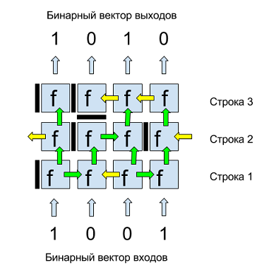
Fig. 1. An example of a binary matrix of 3 rows and 4 binary inputs / outputs.
The structure of the matrix is subject to the rules of a phased line-by-line construction. If this set of neuron rows does not solve the problem, then the following are added to them, and so on until the objective function is reached.
Before learning, the matrix consists of one first row. Learning matrix is to consistently add rows. New lines are added after finding one or more configurations of partitions on the current line, as well as internal parameters of neurons for which the error value on the training sets of the matrix is minimal and less than the value of the training error on the previous line.
Neurons perform the function of converting data, transmitting or stopping the signal. The function of the neuron f , depending on the current configuration of partitions and internal constants, must meet the following mandatory requirements:
1. be able to transfer data without changes;
2. be able to pass a constant (0 or 1) without input data;
3. should not depend on the sequence of application of input data from neighboring neurons, that is, the neuron provides the resulting value from all its inputs received as if simultaneously.
One of the variants of such a function f is modulo 2 addition or exclusive OR or XOR, as it is often denoted in programming languages.
Transmission without change means the actual absence of a neuron and is needed only in terms of transmitting the level of the matrix without changing the data.
Depending on the position (values) of the neuron partitions and its neighboring neurons, each neuron can have from zero to three inputs (bottom, right and left) and always one output (up), which, however, may not be connected to the neuron of the next line , due to the position of the horizontal septum of the upper neuron “stop”.
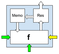
Fig. 2. A neuron with a binary function f , a memory cell Memo and a field Res.
1. The unchanged data transfer is provided by the option shown in Fig. 3. Here Memo = 0, Horizontal lower partition in the meaning of “up”, Left and right partition in the meaning of “stop”.
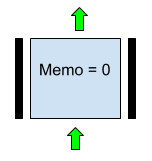
Fig. 3. A variant of the parameters of the neuron that implements the transfer of the input from the previous line without change in the case of f = XOR.
2. The transfer of a constant is provided by the values of the horizontal and vertical “stop” partitions, and the Memo value is the value of the transmitted constant.
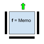
Fig. 4. A neuron with a function that transmits the Memo independent binary constant. Input values from the bottom, left and right are not used.
3. The requirement of independence of the value of the neuron function from the sequence of processing the input values of the neuron is provided by the associativity of XOR.
Sequential, line-by-line construction of the matrix function allows you to effectively optimize the learning process by replacing the complete search through the combinations of binary functions of all neurons of the matrix by a full search of the combinations of functions of neurons of the rows. One of the key points in network training is the number of combinations of complete busting of neuron functions of a single string.
For the variant of the neuron described above, the following functions are involved in the search for the functions of the neuron:
1. horizontal partition with two positions: stop and up;
2. vertical neuron septum with three positions: stop, left and right;
3. Memo binary field with values of 0 and 1.
To calculate the number of variants of neuron functions based on combinations of these parameters, we multiply the number of value options for each of these parameters:
. Thus, each neuron, depending on the number of parameters arriving at the input, can have one of 12 variants of the binary function. Let us calculate the number of variants for the complete enumeration of the functions of one row of a matrix of 8 neurons, which, thus, can process data of 1 byte size: .
For a modern personal computer, this is not a very large number of calculations. When choosing a function of a neuron with a smaller number of options, for example, without a Memo field, the number of combinations significantly decreases to . Even such a significantly simplified version of the neuron function demonstrates a decrease in the learning error in the optimization process. In software tests with different versions of neural functions in C #, the author managed to get the search speed in the range of 200-600 thousand options per second, which gives a complete search through the matrix row functions in about 3 seconds. However, this does not mean that, for example, an 8x8 matrix will be trained within 24 seconds. The fact is that there are several possible variants of the function of a string that give the same current minimum value of a training error (metric). Which of these, tens, hundreds or thousands of combinations will eventually lead to zero learning error of the whole matrix, we do not know, and then in the worst case, we will need to check each of them, which leads to the construction of an optimization search tree.
The function of the learning error matrix will be called the metric. The value of the metric shows the degree of deviation of the output of the matrix from the expected on the training data.
An example of a metric. Suppose that the inputs and outputs of the matrix are 4-bit numbers. And we want to train the matrix to multiply the input numbers by . Assume that three input values are used for learning. , the ideal output for which will be numbers .
The learning process of the matrix consists in the sequential search of the positions of the neuronal partitions and the values of the Memo fields in the neurons of the string, which together serve as search parameters. After each change of one of these parameters, that is, for example, changing the position of the horizontal septum of one of the neurons from the stop position to the up position or changing the Memo field value from 1 to 0, we obtain the current combination of partitions and fields and calculate the value of the metric .
To get the value of the metric on some combination of partitions and Memo fields, we substitute the values of the learning inputs into the matrix and get the outputs.
In this case, the learning error is 5 and the task is to find such a configuration of neurons on the current top row of the matrix, for which the value of the metric is less .
General algorithm for constructing a matrix optimization tree.
The details of this algorithm can be different, both in terms of saving memory and speeding up work, for example, sorting lists due to the peculiarities of matrix neuron partition configurations or discarding previous branch lists in accordance with a decrease in the current metric value.
Practical experiments show that the algorithm for learning the matrix in most cases converges. For example, in one of the tests with the XOR neuron function, an 8-bit matrix learned to multiply by 2 numbers from 1 to 6 with a zero learning error. Substituting at input 7, I got 14 at the output, so the matrix has learned to extrapolate one move ahead, but already at number 8 the matrix gave the wrong result. All training took a few minutes on a personal home computer. However, experiments with more complex training samples require different computational powers.
From flat neurons you can go to three-dimensional, i.e. consider them not as square elements, but as cubes, each face of which receives or transmits data, and then (so far theoretically) you can get a completely tangible three-dimensional artificial brain.
1. AV Kazantsev, VISUAL DATA PROCESSING AND ACTION CONTROL USING BINARY NEURAL NETWORK - IEEE Eighth International Workshop (WIAMIS '07) Image Analysis for Multimedia Interactive Services, 2007.
2. Natalya Efremova, Neural networks: practical application (habrahabr.ru)
3. Functional completeness of Boolean functions (Wikipedia)
Prerequisites for creating a binary matrix neural network
Attempts to create artificial neural networks are based on the fact of the existence of their natural prototypes. The method of transmitting and processing information in the natural neural network is determined by the chemical and biological properties of living neuron cells. However, the model of an artificial neural network does not have to completely copy both the function of the neurons and the structure of the natural brain, since it implements only the function of transforming information inputs into the outputs. Therefore, the implementation of the function of an artificial neural network may differ significantly from its natural counterpart. An attempt to directly copy the structure of the natural brain inevitably encounters the following problems, which, in the absence of their solution, may prove to be insurmountable. As you know, in the mammalian brain, the output of a neuron can be connected to the inputs of several other neurons.
How to know the inputs of which neurons should be connected to the outputs of other neurons? How many neurons should be associated with each specific neuron in the network for the network to perform its function?
There are no answers to these questions yet, and connecting the neurons to each other using a brute force method guarantees an almost infinite time for training such a network, given that the number of real brain neurons is in the billions.
')
In perceptron-type artificial neural networks, all the neurons of adjacent layers are connected to each other. A "strength" of communication is determined by the value of the coefficients. The “all-with-all” connection is the solution of the problem of neuron connections using the “brute force” method. In this case, the neural network can contain only a relatively small number of neurons on the intermediate layers for an acceptable learning time, for example, for several weeks [2].
Before a neural network begins to produce a result, for example, to classify images, it must go through a training phase, that is, a setup phase. At the learning stage, the interaction configuration and the overall function of the neurons of the network are determined. In fact, to train a neural network means to choose a transformation function so that at the given inputs it gives the correct outputs with a given level of error. Then, after training, we give arbitrary data to the network input, and we hope that the neural network function is chosen quite accurately and the network will correctly, from our point of view, classify any other input data. In popular networks of perceptron type, the network structure is initially fixed, see, for example, [2], and the function is found by selecting the neuron connections of the intermediate layers.
The principle of decomposition of several parallel connections into a sequence of pairs or triples of connections of only neighboring neurons forms the basis of the matrix described below. The restriction is accepted that it is not at all necessary to train the network by connecting all the others to the neuron, it suffices to restrict ourselves to neighboring neurons and then consistently reduce the error of the network learning function. This version of the neural network is based on the previous work of the author [1].
The structure of the matrix and neuron
The following matrix structure of the neural network allows to solve the problem of connecting neurons and limit the number of combinations when searching for the function of the neural network. This network also in theory allows us to find the function of a neural network with zero error on the training sets of inputs / outputs due to the fact that the network function is a discrete vector function of several variables.
Figure 1 presents an example of a binary matrix. The inputs and outputs of this matrix are binary four-component vectors. Inputs are given from below, above we get output values. Each matrix cell is a neuron with a binary function of several variables f . Each neuron has horizontal and vertical septa separating it from neighboring neurons and determining the data flows. The vertical partition of the neuron, depicted to the left of each neuron, can have three positions: closed (dark bar), open to the right (green arrow to the right), open to the left (yellow arrow to the left).
The horizontal septum, shown below the neuron, can have two positions: the stop is closed (dark bar) or open up (green arrow). Thus, the data flow in the matrix can be from bottom to top and left / right. In order to avoid allocation of boundary data bits, the first and last neurons in each row are logically looped, that is, for example, the left arrow of the first neuron in a row is the input of the last neuron in the same row, as shown in Figure 1 for neurons of the second row.
Fig. 1. An example of a binary matrix of 3 rows and 4 binary inputs / outputs.
The structure of the matrix is subject to the rules of a phased line-by-line construction. If this set of neuron rows does not solve the problem, then the following are added to them, and so on until the objective function is reached.
Before learning, the matrix consists of one first row. Learning matrix is to consistently add rows. New lines are added after finding one or more configurations of partitions on the current line, as well as internal parameters of neurons for which the error value on the training sets of the matrix is minimal and less than the value of the training error on the previous line.
Neurons perform the function of converting data, transmitting or stopping the signal. The function of the neuron f , depending on the current configuration of partitions and internal constants, must meet the following mandatory requirements:
1. be able to transfer data without changes;
2. be able to pass a constant (0 or 1) without input data;
3. should not depend on the sequence of application of input data from neighboring neurons, that is, the neuron provides the resulting value from all its inputs received as if simultaneously.
One of the variants of such a function f is modulo 2 addition or exclusive OR or XOR, as it is often denoted in programming languages.
Transmission without change means the actual absence of a neuron and is needed only in terms of transmitting the level of the matrix without changing the data.
Depending on the position (values) of the neuron partitions and its neighboring neurons, each neuron can have from zero to three inputs (bottom, right and left) and always one output (up), which, however, may not be connected to the neuron of the next line , due to the position of the horizontal septum of the upper neuron “stop”.
Fig. 2. A neuron with a binary function f , a memory cell Memo and a field Res.
1. The unchanged data transfer is provided by the option shown in Fig. 3. Here Memo = 0, Horizontal lower partition in the meaning of “up”, Left and right partition in the meaning of “stop”.
Fig. 3. A variant of the parameters of the neuron that implements the transfer of the input from the previous line without change in the case of f = XOR.
2. The transfer of a constant is provided by the values of the horizontal and vertical “stop” partitions, and the Memo value is the value of the transmitted constant.
Fig. 4. A neuron with a function that transmits the Memo independent binary constant. Input values from the bottom, left and right are not used.
3. The requirement of independence of the value of the neuron function from the sequence of processing the input values of the neuron is provided by the associativity of XOR.
The number of combinations of a full brute force function string
Sequential, line-by-line construction of the matrix function allows you to effectively optimize the learning process by replacing the complete search through the combinations of binary functions of all neurons of the matrix by a full search of the combinations of functions of neurons of the rows. One of the key points in network training is the number of combinations of complete busting of neuron functions of a single string.
For the variant of the neuron described above, the following functions are involved in the search for the functions of the neuron:
1. horizontal partition with two positions: stop and up;
2. vertical neuron septum with three positions: stop, left and right;
3. Memo binary field with values of 0 and 1.
To calculate the number of variants of neuron functions based on combinations of these parameters, we multiply the number of value options for each of these parameters:
. Thus, each neuron, depending on the number of parameters arriving at the input, can have one of 12 variants of the binary function. Let us calculate the number of variants for the complete enumeration of the functions of one row of a matrix of 8 neurons, which, thus, can process data of 1 byte size: .
For a modern personal computer, this is not a very large number of calculations. When choosing a function of a neuron with a smaller number of options, for example, without a Memo field, the number of combinations significantly decreases to . Even such a significantly simplified version of the neuron function demonstrates a decrease in the learning error in the optimization process. In software tests with different versions of neural functions in C #, the author managed to get the search speed in the range of 200-600 thousand options per second, which gives a complete search through the matrix row functions in about 3 seconds. However, this does not mean that, for example, an 8x8 matrix will be trained within 24 seconds. The fact is that there are several possible variants of the function of a string that give the same current minimum value of a training error (metric). Which of these, tens, hundreds or thousands of combinations will eventually lead to zero learning error of the whole matrix, we do not know, and then in the worst case, we will need to check each of them, which leads to the construction of an optimization search tree.
Building an optimization tree or finding zero learning matrix errors
The function of the learning error matrix will be called the metric. The value of the metric shows the degree of deviation of the output of the matrix from the expected on the training data.
An example of a metric. Suppose that the inputs and outputs of the matrix are 4-bit numbers. And we want to train the matrix to multiply the input numbers by . Assume that three input values are used for learning. , the ideal output for which will be numbers .
The learning process of the matrix consists in the sequential search of the positions of the neuronal partitions and the values of the Memo fields in the neurons of the string, which together serve as search parameters. After each change of one of these parameters, that is, for example, changing the position of the horizontal septum of one of the neurons from the stop position to the up position or changing the Memo field value from 1 to 0, we obtain the current combination of partitions and fields and calculate the value of the metric .
To get the value of the metric on some combination of partitions and Memo fields, we substitute the values of the learning inputs into the matrix and get the outputs.
In this case, the learning error is 5 and the task is to find such a configuration of neurons on the current top row of the matrix, for which the value of the metric is less .
General algorithm for constructing a matrix optimization tree.
1. , max(Int32). , "" Memo. 2. : . a. , , , . b. , . c. , , . d. , ( ) . 3. , . The details of this algorithm can be different, both in terms of saving memory and speeding up work, for example, sorting lists due to the peculiarities of matrix neuron partition configurations or discarding previous branch lists in accordance with a decrease in the current metric value.
Conclusion
Practical experiments show that the algorithm for learning the matrix in most cases converges. For example, in one of the tests with the XOR neuron function, an 8-bit matrix learned to multiply by 2 numbers from 1 to 6 with a zero learning error. Substituting at input 7, I got 14 at the output, so the matrix has learned to extrapolate one move ahead, but already at number 8 the matrix gave the wrong result. All training took a few minutes on a personal home computer. However, experiments with more complex training samples require different computational powers.
From flat neurons you can go to three-dimensional, i.e. consider them not as square elements, but as cubes, each face of which receives or transmits data, and then (so far theoretically) you can get a completely tangible three-dimensional artificial brain.
Links
1. AV Kazantsev, VISUAL DATA PROCESSING AND ACTION CONTROL USING BINARY NEURAL NETWORK - IEEE Eighth International Workshop (WIAMIS '07) Image Analysis for Multimedia Interactive Services, 2007.
2. Natalya Efremova, Neural networks: practical application (habrahabr.ru)
3. Functional completeness of Boolean functions (Wikipedia)
Source: https://habr.com/ru/post/343304/
All Articles