Slight discrepancy

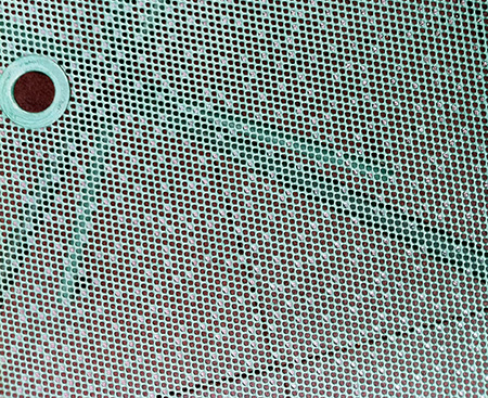
This picture shows a mesh table top on a patio, photographed after a heavy rain. In some of the mesh holes lingered water drops. What can be said about the distribution of these drops? Are they scattered randomly on the surface? The process of falling rain, which has arranged them, seems to be quite random, but in my opinion, the pattern of places occupied in the grid looks suspiciously even and monotonous.



To simplify the analysis, I selected the square part of the photograph with the table top (removing the hole for the umbrella), and selected the coordinates of all the drops in this square. There are 394 drops in it, which I marked with blue dots:

')





I will repeat the question: does this pattern look like a result of a random process?



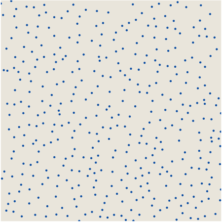
I came to this question after writing an article for American Scientist , in which two variants of simulated randomness are studied: pseudo and quasi . Pseudo-randomness needs no introduction. A pseudo-random algorithm for selecting points in a square tends to ensure that all points have the same probability of choice, and that all choices are independent of each other. Here is an array of 394 pseudo-random points bounded by belonging to a beveled and rotated grid, similar to a mesh table top:







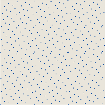
Quasi-randomness is a less well-known concept. When choosing quasi-random points, the goal is not equiprobability or independence, but the uniformity of the distribution: the scatter of the points as evenly as possible over the surface of the square. However, it is not too obvious how to achieve this goal. For the 394 quasi-random points shown below, the x coordinates form a simple arithmetic progression, but the y coordinates are altered by the process of mixing numbers. (The corresponding algorithm was invented in the 1930s by the Dutch mathematician Johannes van der Korput, who worked on one-dimensional rows, and in the 1950s was transferred to two dimensions by Klaus Friedrich Roth. For more details, see my article for American Scientist on page 286 or in an amazing book Jiri Matusek .)







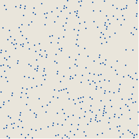
Which of these sets of points, pseudo or quasi , best fits raindrops? We can compare all three patterns in a reduced form:







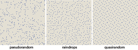
Each of the patterns has its own texture. In a pseudo-random, there are both concentrated clusters and large spaces. Quasi-random points are located more evenly (although there are several close pairs of points), but they also create distinct small-scale repeating patterns, the most prominent of which is the hexagonal structure, repeated with almost crystalline uniformity. As for the drops, it looks like they are distributed over the area with almost uniform density (in this resembling a quasi-random pattern), but in the texture there are hints of bends rather than lattices (in this case it looks more like a pseudo-random example).



Instead of studying patterns "by eye", you can try a quantitative approach to their description and classification. For this purpose, there are many tools: radial distribution functions, statistics of nearest neighbors, Fourier methods, but the main reason for solving this issue for me was first of all the opportunity to play with a new toy, which I learned in the process of studying quasi-randomness. This quality, called discrepancy, could not find the correct term in Russian, so write to me if you know it , estimates the deviation of the set of points from the uniform distribution in space.



There are many variations in the concept of discrepancy, but I want to consider only one measurement scheme. The idea is to overlay on a pattern of rectangles of various shapes and sizes, the sides of which are parallel to the x and y axes. Here are three examples of rectangles superimposed on a droplet pattern:







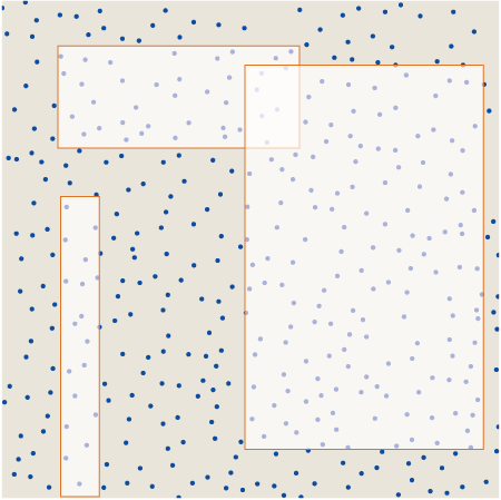
Now we calculate the number of points enclosed in each rectangle, and compare them with the number of points that should be enclosed in it with a corresponding area, if the distribution of points was perfectly uniform over the whole square. The absolute value of the difference is the difference $$$D (r)$ associated with a rectangle $$$R$ :

$$

$$D \ left (R \ right) = \ left | N \ cdot area (R) - \ # \ left (P \ cap R \ right) \ right |$$

Where $$$N$ - the total number of points, and $$$\ # \ left (P \ cap R \ right)$ - amount of points $$$P$ in a rectangle $$$R$ . For example, the rectangle in the upper left corner covers 10 percent of the square, that is, its “fair” share of points should be 0.1 × 394 = 39.4 points. In fact, the rectangle contains only 37 points, that is, the discrepancy associated with the rectangle is | 39.4 - 37 | = 2.4. The density of points in a rectangle can be more or less than the general average; in both cases, the absolute value will give us a positive discrepancy.



For the pattern as a whole, we can set the total discrepancy D as the worst value of its change, or in other words, the maximum discrepancy taken for all possible rectangles superimposed on a square. Van der Korput wondered if the sets of points could be created with an arbitrarily low divergence, so that $$$N$ tending to infinity $$$D$ has always been below some fixed boundary. The answer is no, in at least one and two dimensions; minimum growth rate is $$$O \ left (\ log N \ right)$ . Pseudo-random patterns generally have a higher discrepancy $$$O \ left (\ sqrt {N} \ right)$ .



How to find a rectangle with the maximum divergence for a given set of points? When I first read the definition of discrepancy, I thought that it would be impossible to calculate it precisely, because there are an infinite number of rectangles in question. But upon reflection, I realized that there was only a finite set of candidate rectangles that could maximize the divergence. These are rectangles in which each of the four sides passes through at least one point. (Exception: candidate rectangles may also have sides lying on the edges of a square.)



Suppose we meet the following rectangle:







The left, upper and lower sides pass through the point ,, but the right side lies in “empty space”. Such a configuration cannot be a rectangle with a maximum divergence. We can move the right edge to the left until it intersects with a point:







This change in shape reduces the area of ​​the rectangle without changing the number of points enclosed in it, and therefore increases the density of points. We can also move the edge in the other direction:







Now we have increased the area, again without changing the number of points enclosed in it, which means we have reduced the density. At least one of these actions will increase $$$D (r)$ compared to the original configuration. Therefore, each rectangle, all four sides of which touch points or edges of a square, is a local maximum of the divergence function; by listing all the rectangles in this finite set, we can find the global maximum.



There is also another annoying question: should a rectangle be considered “closed” (that is, points on the border are included in the area) or “open” (points on the borders are excluded). I avoided this task by presenting in the form of a table the results for both closed and open borders. The closed form gives the greatest discrepancy for rectangles with a dense arrangement of points, and the open form maximizes the divergence at a low density of points.



Considering only the extremes of the divergence function, we make the calculation task finite - but everything is not so simple! How many rectangles need to be considered in the square with $$$N$ points (each of which has its own distinct coordinates $$$x$ and $$$y$ )? This turns out to be a very interesting little task with a simple combinatorial solution. I will not explain the answer here, but if you don’t think you can do it yourself, you can watch it in OEIS or read the short article by Benjamin, Quinn and Wurtz . What I can say is that for N = 394 the number of rectangles is 6,055,174,225 — or two times more, if we separately take into account open and closed rectangles. For each rectangle, you need to find out how many of the 394 points are inside and how many are outside. Quite a lot of work.



One way to reduce computational overhead is to return to a simpler measurement of the discrepancy. In different literature on quasi-random patterns in two or more dimensions, a quality called “star discrepancy”, or D *, is used . The idea is to consider only rectangles “attached” to the lower left corner of the square (which successfully coincides with the origin point of the xy plane). In this case, the number of rectangles is equal to $$$N ^ {2}$ , or about 150,000 for N = 394.



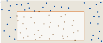
Here is a rectangle defining the global divergence-star of the raindrop pattern:







The dark green box at the bottom covers about 55 percent of the square and should contain 216.9 dots with a completely even distribution. In fact, it includes (assuming that this is a “closed” rectangle) 238 points, that is, the discrepancy is 21.1. No other rectangle tied to a corner (0,0) will have more divergence. (Note: due to the limitations of the graphic resolution, it seems that the rectangle D * stretches to the bounds of the square, in fact the right edge lies on x = 0.999395.)



What does this result tell us about the nature of the raindrop pattern? Well, for starters, the discrepancy is pretty close to $$$\ sqrt {N}$ (equivalent to 19.8 with N = 394) and not particularly close to $$$\ log N$ (equal to 6.0 for natural logarithms). That is, we do not find evidence that the droplet pattern is more quasi-random than pseudo-random. The values ​​of D * for the other patterns shown above are in the expected interval: 25.9 for pseudo-random and 4.4 for quasi-random. In contrast to the external impression, the distribution of raindrops seems to have more in common with a pseudo-random set of points than with a quasi-random - at least according to the criterion D * .



But what about the calculation of the unlimited divergence D , that is, the study of all rectangles, and not just fixed rectangles D * ? Upon reflection, it can be concluded that a comprehensive enumeration of rectangles cannot in this case change the main conclusion; D can never be less than D * , and therefore we cannot hope to approach from $$$\ sqrt {N}$ to $$$\ log N$ . But I was still interested in calculations. Which of all these six billion rectangles will have the largest discrepancy? Is it possible to answer this question without heroic feats?



The obvious and simple algorithm for D generates in turn all the candidate rectangles, measures their area, counts points inside and tracks the marginal differences found in the process. I found out that a program that implements this algorithm can determine the exact discrepancy of 100 pseudo-random or quasi-random points in a few minutes. This result may motivate us to take large N values; however, the execution time almost doubles each time N is increased by 10, and this hints to us that for N = 394 calculations will take a couple of centuries.



I spent a few days trying to speed up the calculations. Most of the execution time is spent on a procedure that counts points in each rectangle. Determining whether a given point is inside, outside or on the border takes eight arithmetic comparisons; that is, when N = 394, more than 3,000 are executed for each of the six billion rectangles. The most effective method of saving time I discovered was the preliminary calculation of all comparisons. For each point that may become the lower left corner of the rectangle, I first calculate the list of all points of the pattern that are above and to the right. For each potential upper right corner of the rectangle, I compile a similar list of points below and to the left. These lists are stored in a hash table indexed by angle coordinates. For each triangle, I can calculate the number of interior points by simply taking the intersection of the sets of two lists.



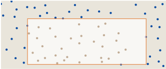
Thanks to this trick, the expected execution time with N = 394 decreases from two centuries to about two weeks. This great optimization encouraged me to spend another day on further improvements. The situation of replacing the hash table with an N × N array slightly improved the situation. And then I found a way to ignore all the smallest triangles that are not likely to be rectangles with maximum D , because they contain too few points, or they have too small an area. This improvement has finally reduced the lead time to one night. It took six hours to calculate an illustration showing a rectangle with a maximum divergence D for a raindrop pattern.







The rectangle with max- D obviously became a small refinement of the rectangle D * for the same set of points. The rectangle D “must” contain 204.3 points, but in fact contains 229, which gives us the difference D = 24.7. Of course, the knowledge that the exact discrepancy is 24.7, not 21.1, does not tell us anything about the nature of the raindrop pattern itself. In fact, it seems to me that by doing more and more calculations, I find out less and less about it.



When I started working on this project, I had my own theory about what could happen in the table top to smooth out the distribution of drops and what makes the pattern more quasi- than pseudo-random. For a start, I thought about the drops lying on the smooth surface of the glass, and not the metal grid. If two small drops are close enough to touch, they will merge into one large drop, because this configuration has less energy associated with surface tension. If two adjacent cells of the grid are filled with water, and if the metal between them is wet, then water can flow freely from one drop to another. A larger drop will almost certainly grow at the expense of a smaller one, and the latter will eventually disappear. Therefore, compared to a purely random distribution, we can expect a lack of droplets in neighboring cells.



And this thought still seems to me very good. The only problem is that it explains the phenomenon, which may not exist. I don’t know if my calculations revealed something important about these three patterns, but at least it was not possible to prove by measurements that the distribution of drops differs from the pseudo-random. In fact, the patterns look different, but how much can we trust our organs of perception in such cases? If you ask people to draw dots at random, the majority will handle this badly, usually the distribution will be too smooth and even. Perhaps the brain is experiencing similar difficulties in recognizing chance.



However, I believe that there is some mathematical property that allows you to more effectively separate these patterns. If someone else decides to spend their time searching, the xy coordinates for the three sets of points are in the text file .



Update : this is just a brief recommendation - if you have read this far, then continue reading the comments . They have a lot of value. I want to thank all those who have spent their time to offer alternative explanations or algorithms and to point out weak points in my analysis. Special thanks to themathsgeek, who 40 minutes after publishing the post wrote a much better program for calculating discrepancies. I also thank Iain, who checked my improvised reasoning about the perception of random patterns with real experiments.