Visualization of the neural network learning process using TensorFlowKit

Starting working in the field of machine learning, it was hard for me to move from objects and their behaviors to vectors and spaces. At first, all this was rather hard in the head and far from all the processes seemed transparent and understandable at first glance. For this reason, I tried to visualize everything that was happening inside my work: I built 3D models, graphs, charts, images, and so on.



Speaking about the effective development of machine learning systems, there is always the issue of controlling the speed of learning, analyzing the learning process, collecting various learning metrics, and so on. The particular difficulty lies in the fact that we (people) are used to operating with 2 and 3 dimensional spaces, describing various processes around us. Processes inside neural networks occur in multidimensional spaces, which seriously complicates their understanding. Realizing this, engineers around the world are trying to develop different approaches to visualizing or transforming multidimensional data into simpler and more understandable forms.



There are entire communities that solve such tasks, for example Distill , Welch Labs , 3Blue1Brown .

Tensorboard

Before I started working with TensorFlow, I started working with the TensorBoard package. It turned out that this is a very convenient, cross-platform solution for visualizing various kinds of data. It took a couple of days to “teach” the swift application to create reports in the TensorBoard format and integrate it into my neural network .

')

Development TensorBoard began in mid-2015 in one of the laboratories Google. At the end of 2015, Google opened the source code and the work on the project became public.

The current version of TensorBoard is a python package created to help TensorFlow, which allows you to visualize several data types:

• Scalar data in terms of time, with the possibility of smoothing;
• Images, in the event that your data can be presented in 2D, for example: convolutional network weights (they are filters);
• Directly graph calculations (in the form of an interactive presentation);
• 2D change of the tensor value in time;
• 3D Histogram - change in the distribution of data in the tensor in time;
• Text;
• Audio;

In addition, there is also a projector (projector) and the ability to extend TensorBoard with the help of plug-ins , but I will not have time to tell about this in this article.



To work we need TensorBoard on our computer (Ubuntu or Mac). We need to have python3 installed. I suggest installing TensorBoard as part of the TensorFlow package for python.

Linux: $ sudo apt-get install python3-pip python3-dev $ pip3 install tensorflow MacOS: $ brew install python3 $ pip3 install tensorflow 

Run TensorBoard, specifying the folder in which we will store the reports:

 $ tensorboard --logdir=/tmp/example/ 

http://localhost:6006/



TensorFlowKit

GitHub example

Do not forget to put the "start" repository.



Let us consider several cases directly on an example. Creation of reports (summary) in the TensorBoard format occurs at the moment of constructing the calculation graph. In TensorFlowKit, I tried to repeat as much as possible the python approaches and interface, so that in the future you could use the general documentation.



As I said above, we collect each report in summary. This is the container in which the value array is stored, each of which represents an event that we want to visualize.



Summary will be saved to a file on the file system, where TensorBoard will read it.







Thus, we need to create a FileWriter by specifying the graph that we want to visualize and create a Summary into which we will add our values.

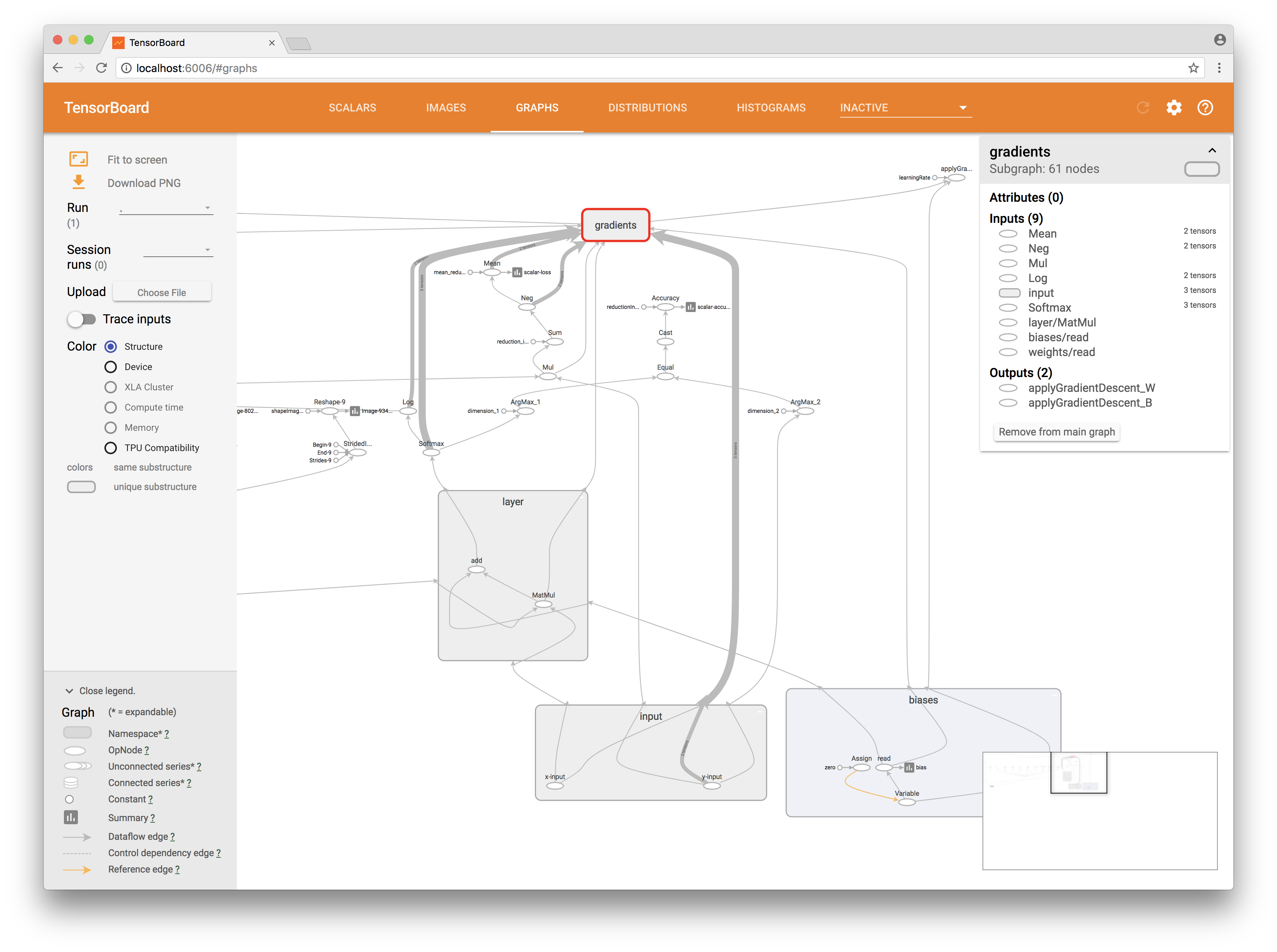
 let summary = Summary(scope: scope) let fileWriter = try FileWriter(folder: writerURL, identifier: "iMac", graph: graph) 

By running the application and refreshing the page, we can already see the graph we created in the code. It will be interactive, so you can navigate through it.







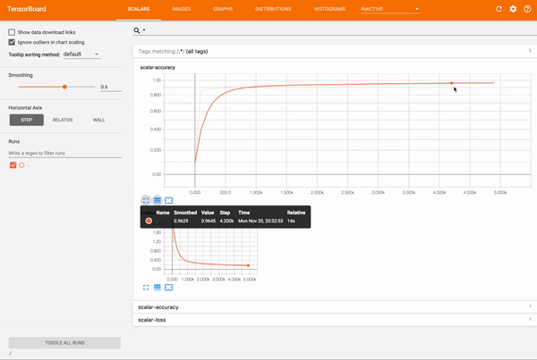
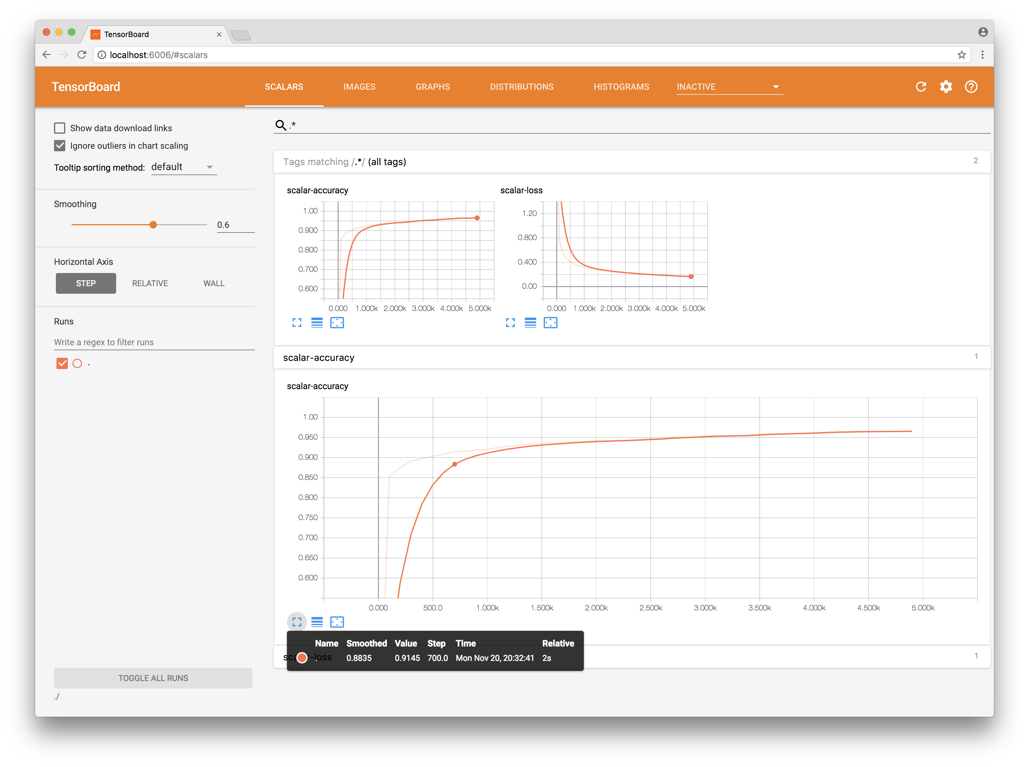
Next, we want to see a change in a certain scalar value over time, for example, the value of the loss function or cost function and accuracy of our neural network. To do this, add the outputs of our operations to the summary:

 try summary.scalar(output: accuracy, key: "scalar-accuracy") try summary.scalar(output: cross_entropy, key: "scalar-loss") 

Thus, after each step of computing our session, TensorFlow automatically subtracts the values ​​of our operations and passes them to the input of the resulting Summary, which we will save in FileWriter (how to do this, I will describe below).







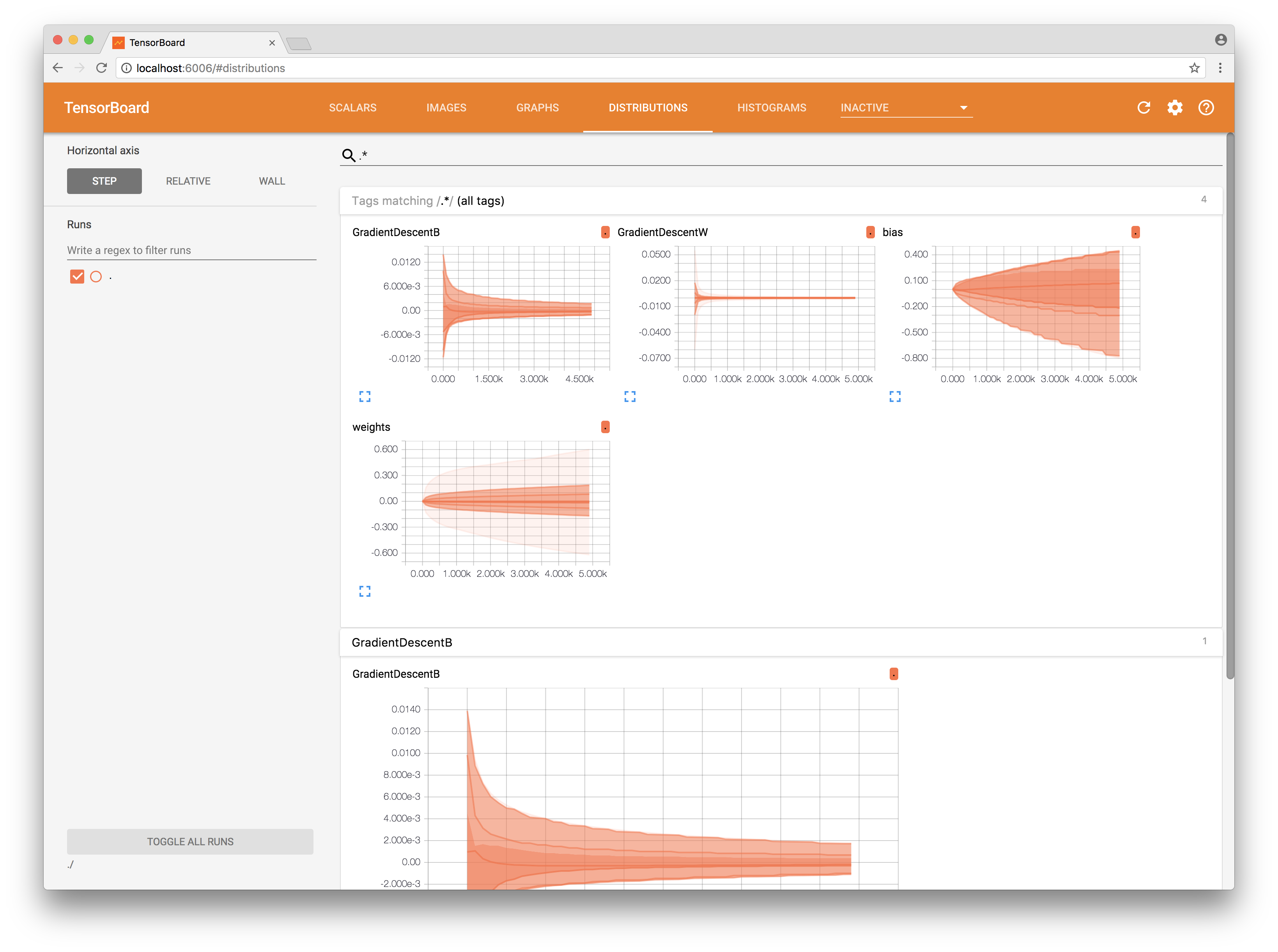
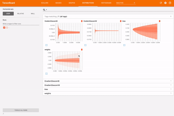
We also have a greater number of weights and biases in the neural network (bias). As a rule, these are various matrices of a rather large dimension and it is extremely difficult to analyze their values ​​when printing. It will be better if we build a distribution schedule. We also add to our Summary information about the magnitude of changes in weights that our network makes after each step of training.

 try summary.histogram(output: bias.output, key: "bias") try summary.histogram(output: weights.output, key: "weights") try summary.histogram(output: gradientsOutputs[0], key: "GradientDescentW") try summary.histogram(output: gradientsOutputs[1], key: "GradientDescentB") 

Now we have at our disposal a visualization of how the weights changed and what the changes were during the training.











But that is not all. Let's really take a look at the device of our neural network.

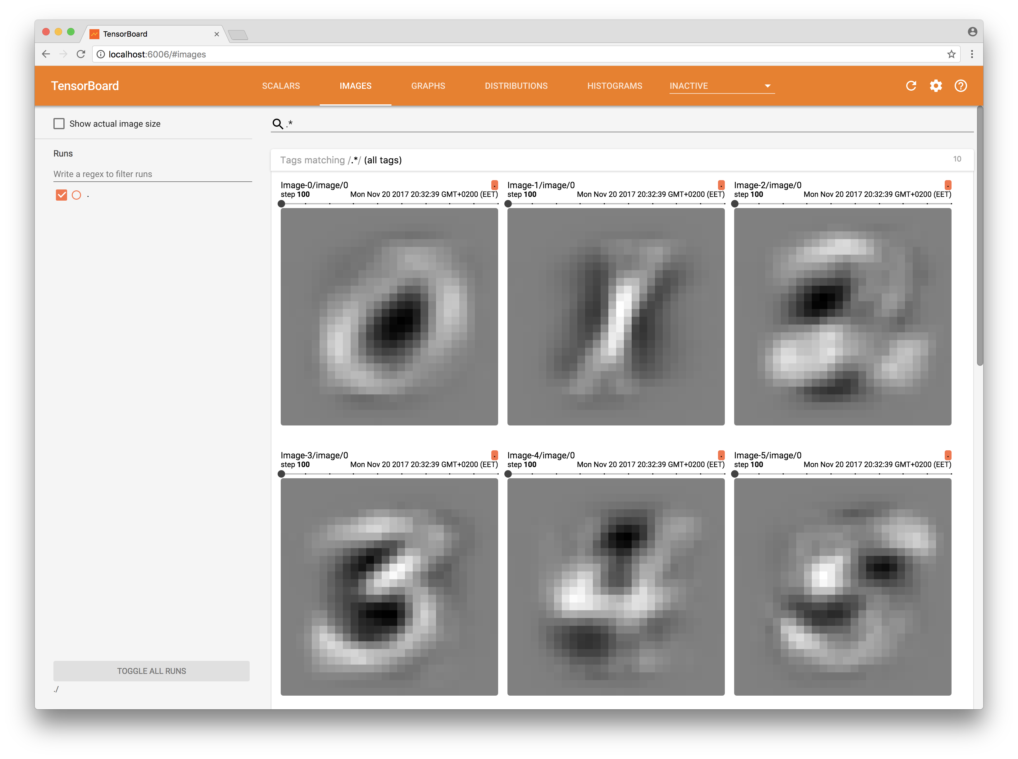
Each picture of the handwritten text received at the entrance is reflected in its corresponding weights. That is, the picture submitted to the input can activate certain neurons, thereby having a certain imprint inside our network. Let me remind you that we have 784 weights for each neuron out of 10. Thus, we have 7840 weights. All of them are presented in the form of a matrix 784x10. Let's try to expand the entire matrix into a vector and then “pull out” the weights that belong to each individual class:

 let flattenConst = try scope.addConst(values: [Int64(7840)], dimensions: [1], as: "flattenShapeConst") let imagesFlattenTensor = try scope.reshape(operationName: "FlattenReshape", tensor: weights.variable, shape: flattenConst.defaultOutput, tshape: Int64.self) try extractImage(from: imagesFlattenTensor, scope: scope, summary: summary, atIndex: 0) try extractImage(from: imagesFlattenTensor, scope: scope, summary: summary, atIndex: 1) … try extractImage(from: imagesFlattenTensor, scope: scope, summary: summary, atIndex: 8) try extractImage(from: imagesFlattenTensor, scope: scope, summary: summary, atIndex: 9) 

To do this, add a few more operations stridedSlice and reshape to the graph. Now, add each received vector to the Summary as an image:

 try summary.images(name: "Image-\(String(index))", output: imagesTensor, maxImages: 255, badColor: Summary.BadColor.default) 

In the Images section of TensorBoard, we now see the “prints” of the weights, as they were during the learning process.







It remains only to process our Summary. To do this, we need to combine all created Summary into one and process it during network training.

 let _ = try summary.merged(identifier: "simple") 

At the time of our network:

 let resultOutput = try session.run(inputs: [x, y], values: [xTensorInput, yTensorInput], outputs: [loss, applyGradW, applyGradB, mergedSummary, accuracy], targetOperations: []) let summary = resultOutput[3] try fileWriter?.addSummary(tensor: summary, step: Int64(index)) 

Please note that in this example I do not consider the issue of calculating accuracy, it is calculated on the training data. Calculate it on the data for learning is wrong.











In the next article I will try to tell you how to build one neural network and run it on Ubuntu, MacOS, iOS from one repository.