Quadratic arithmetic programs: from mud to riches (translation)

Continuing the series of articles on zk-SNARKs technology, we are studying a very interesting article by Vitalik Buterin " Quadratic Arithmetic Programs: from Zero to Hero "

Previous article: Introduction to zk-SNARKs with examples (translation)

Recently, interest in zk-SNARKs has grown immensely, and people are increasingly trying to demystify what many have come to call “lunar math” because of their rather indiscriminate complexity. zk-SNARKs are really quite difficult to understand, especially because of the large number of components that need to be put together to make it all work, but if we disassemble the technology in parts, it will be much easier to comprehend it ...

The purpose of this publication is not a full introduction to the zk-SNARK technology. It is also assumed that, firstly, you know what zk-SNARKs are and what they do, and secondly, you know mathematics well enough to be able to talk about things like polynomials (if the statement P(x) + Q(x) = (P + Q)(x) , where P and Q are polynomials, it seems natural and obvious to you, then your level is sufficient). Rather, this publication reveals the mechanism behind the technology and tries to explain, as far as possible, the first half of the transformations shown by zk-SNARKs researcher Eran Tromer (Eran Tromer):

Conversions here can be divided into two components. First, zk-SNARKs cannot be directly applied to any computational problem; first you need to convert the task to the correct “form” for the problem it solves. A form is called a “quadratic arithmetic program” (QAP), and the transformation of the function code into such a form is in itself a very nontrivial task. Along with converting the function code to QAP, there is another separate action that is performed if you have an input argument for the function to be converted. You need to create an appropriate solution (sometimes called a "certificate" for QAP). There is also another rather complex mechanism for creating an actual “proof with zero disclosure” for this evidence and a separate process for verifying the evidence that was passed to you, but this is a separate conversation beyond the scope of this publication. (For an understanding of the general scheme of the process, see the first article . Comment. Translator).

We will analyze a simple example: it is necessary to prove that you know the solution of a cubic equation:

$$

$$x ^ 3 + x + 5 = 35$$

(hint: answer 3). This task is quite simple, so the resulting QAP will not be so big as to scare you. But the code will be nontrivial enough so that you can see all the math in action.

We describe our function as follows:

 def qeval(x): y = x**3 return x + y + 5 

The simple special-purpose programming language used here supports basic arithmetic ( +, -, *, / ), limited exponentiation ( x**7 , but not x**y ), and assignment to variables, which is quite a powerful tool, allowing you to theory to perform calculations inside the function (as long as the number of calculation steps is limited and cycles are not allowed). Note that modulo division ( % ) and comparison operators ( <,>, ≤, ≥ ) are not supported, as there is no effective way to produce division by modulus or comparison directly in the complete cyclic group arithmetic (be grateful for this, because if there was a way to implement one of these operations, cryptography on elliptic curves would be cracked faster than you would say “binary search” and “Chinese remainder theorem”).

You can extend the language to modulus and comparisons using bit decomposition, for example:

$$

$$13 = 2 ^ 3 + 2 ^ 2 + 1$$

as auxiliary parameters, checking the correctness of these expansions and performing mathematics in binary operations; in the arithmetic of a finite field, checking equality (==) is also feasible and even much easier, but we will not deal with these things now. We can extend the language to support conditional expressions (for example, if x < 5: y = 7; else: y = 9 ) by transforming them into an arithmetic form y = 7 * (x < 5) + 9 * (x >= 5); but note that in this case both branches of the conditional expression must be fulfilled, and if you have a lot of nested conditions, this will lead to an increase in overhead costs.

Let's now go through the conversion process in QAP step by step. If you want to do it yourself for any code, I implemented the compiler here (only for educational purposes, and it is not yet ready to create QAP for real zk-SNARKs!).

Simplify

The first step is the “simplify” procedure. In it, we convert the source code, which can contain an arbitrary number of complex operators and expressions, into a sequence of operators that have two forms:
x = y (where y can be a variable or a number) and
x = y (op) z (where op can be +, -, *, / ; y and z can be variables, numbers, or subexpressions).

You can think of each of these operators as a logical transition in a circuit (meaning "logic gate", changing states. Approx. Translator). The result of the simplification process for the above code is the following:

 sym_1 = x * x y = sym_1 * x sym_2 = y + x ~out = sym_2 + 5 

If you look at the source code and the code above, you can easily see that they are equivalent.

Transition to R1CS

Now we will transform this into what is called a "Rank-1 Restriction System" (R1CS). R1CS is a sequence of groups of three vectors (a, b, c), and the solution R1CS is a vector s , where s must satisfy the equation sa * sb - sc = 0 , where . is a "taking a point" (multiplying a row vector by a column vector. Approx. translator) . In simple terms, if we “combine” a and s , multiplying the values ​​of vectors in the same positions, and then take the sum of these products, then do the same for b and, s and then, the same for c and s then the third result will be equal to the product of the first two results. Example of R1CS solution:
')

But instead of having only one restriction in the program, we introduce a set of restrictions: one for each logical transition. There is a standard way of converting a logical transition to (a, b, c) triplet, depending on which operation is performed (+, -, * or /), and whether the arguments are variables or numbers. The length of each vector is equal to the total number of variables in the system, which includes the dummy variable ~one in having a value of 1, the input parameters, the dummy variable ~out representing the result, as well as all intermediate variables ( sym1 and sym2 see above); Vectors, as a rule, will be very “sparse”, with filled values ​​corresponding to variables that are affected by a particular logical transition.

Let's denote the list of variables that we will use:
'~one', 'x', '~out', 'sym_1', 'y', 'sym_2'

The solution vector will consist of assigning values ​​for all of these variables in a similar order.

Now we will find (a, b, c) three for the first transition:

 a = [0, 1, 0, 0, 0, 0] b = [0, 1, 0, 0, 0, 0] c = [0, 0, 0, 1, 0, 0] 

It is easy to make sure that if the value of the solution vector in the second position is 3, and in the fourth position is 9, then regardless of the other values ​​of the solution vector, the vector check will be reduced to 3*3 = 9 and the solution will be correct. If the value of the solution vector is -3 in the second position and 9 in the fourth, then the verification will also be successful. The same is true for the value 7 in the second position and 49 in the fourth. The purpose of this first check is to make sure that only the first transition only has inputs and outputs.

Now let's go to the second transition:

 a = [0, 0, 0, 1, 0, 0] b = [0, 1, 0, 0, 0, 0] c = [0, 0, 0, 0, 1, 0] 

Similar to the first check, here we check sym_1 * x = y

Third transition:

 a = [0, 1, 0, 0, 1, 0] b = [1, 0, 0, 0, 0, 0] c = [0, 0, 0, 0, 0, 1] 

Here, the pattern is somewhat different: it multiplies the first element in the solution vector by the second element, then by the fifth element, adding two results and checking whether the sum is equal to the sixth element. Since the first element in the solution vector is always equal to one, this is just an addition check, confirming that the output is equal to the sum of the two inputs.

Finally, the fourth transition:

 a = [5, 0, 0, 0, 0, 1] b = [1, 0, 0, 0, 0, 0] c = [0, 0, 1, 0, 0, 0] 

Here we reproduce the last check ~out = sym_2 + 5 . The test works by taking the sixth element in the solution vector, adding the first element multiplied by 5 (recall: the first element is 1, so this actually means adding 5) and relating it to the third element where we store the output variable.

So, we have R1CS with four limitations. The evidence is simply the value of all variables, including input, output, and internal variables:

 [1, 3, 35, 9, 27, 30] 

You can calculate it yourself by simply “executing” the simplified code above, starting with assigning the input variables x = 3, entering the values ​​of all intermediate variables and changing them during the calculation.

Now we give the full R1CS for our case:

 A [0, 1, 0, 0, 0, 0] [0, 0, 0, 1, 0, 0] [0, 1, 0, 0, 1, 0] [5, 0, 0, 0, 0, 1] B [0, 1, 0, 0, 0, 0] [0, 1, 0, 0, 0, 0] [1, 0, 0, 0, 0, 0] [1, 0, 0, 0, 0, 0] C [0, 0, 0, 1, 0, 0] [0, 0, 0, 0, 1, 0] [0, 0, 0, 0, 0, 1] [0, 0, 1, 0, 0, 0] 

R1CS - QAP

The next step is to convert this R1CS to a QAP form, which implements the same logic, but polynomials will be used instead of taking a point. We will do this as follows: we will move from four groups of three vectors of six lengths to six groups of three 3rd degree polynomials, where each x coordinate of the polynomial corresponds to one of the constraints. That is, if we calculate the values ​​of the polynomials at x = 1, then we get our first set of vectors, if we calculate the polynomials from x = 2, then we get the second set of vectors, etc.

We can do this transformation using, for example, the Lagrange interpolation polynomial. The problem that Lagrange interpolation solves is as follows: if you have a set of points (ie (x, y) coordinate pairs), then performing Lagrange interpolation at these points gives you a polynomial passing through all these points. We do this by breaking the task as follows: for each value of x we create a polynomial that returns y value corresponding to the given point (x, y) and returns 0 in all other cases. And then, to get the final result, we add all the polynomials.

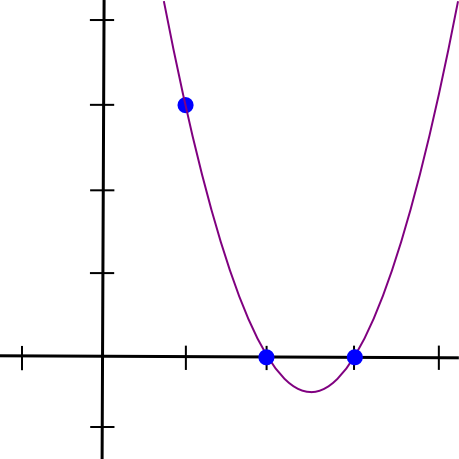
Let's give an example. Suppose we need a polynomial passing through (1, 3), (2, 2) and (3, 4). We start by creating a polynomial passing through (1, 3), (2, 0) and (3, 0). As it turned out, to make a polynomial that takes a value only for x = 1 and is equal to zero in other cases is very simple:

 (x - 2) * (x - 3) 

On the graph it looks like this:

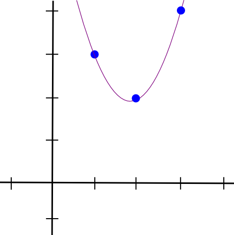
Now we just need to "zoom" in order for the height at the point x = 1 to be necessary:

 (x - 2) * (x - 3) * 3 / ((1 - 2) * (1 - 3)) 

This will give us:

$$

$$1.5 * x ^ 2 - 7.5 * x + 9$$

Then we do the same thing with two other points and get two other similar polynomials, except that they take values ​​for x = 2 and x = 3 instead of x = 1.

We add all three polynomials together and get:

$$

$$1.5 * x ^ 2 - 5.5 * x + 7$$

This is exactly what we need. The complexity of the execution time of the above algorithm is O (n^3) , since there are n points, and each point requires O (n^2) time to multiply the polynomials. By optimizing a bit, complexity can be reduced to O (n^2) . And if you use fast Fourier transform algorithms, etc., the complexity can still be reduced - this significantly optimizes zk-SNARKs, since in practice, real functions can contain thousands of transitions.

Now let's convert our R1CS to the Lagrange interpolation polynomial. We take the value of the first position from each vector a , apply the Lagrange interpolation to get a polynomial (where the calculation of the value of the polynomial at the point i will give the value of the ith vector a in the first position). Then repeat the process for the value of the first position of each vector b and c , and then repeat this process for subsequent positions. For convenience, I will show you the result immediately:

  A [-5.0, 9.166, -5.0, 0.833] [8.0, -11.333, 5.0, -0.666] [0.0, 0.0, 0.0, 0.0] [-6.0, 9.5, -4.0, 0.5] [4.0, -7.0, 3.5, -0.5] [-1.0, 1.833, -1.0, 0.166]  B [3.0, -5.166, 2.5, -0.333] [-2.0, 5.166, -2.5, 0.333] [0.0, 0.0, 0.0, 0.0] [0.0, 0.0, 0.0, 0.0] [0.0, 0.0, 0.0, 0.0] [0.0, 0.0, 0.0, 0.0]  C [0.0, 0.0, 0.0, 0.0] [0.0, 0.0, 0.0, 0.0] [-1.0, 1.833, -1.0, 0.166] [4.0, -4.333, 1.5, -0.166] [-6.0, 9.5, -4.0, 0.5] [4.0, -7.0, 3.5, -0.5] 

The coefficients are sorted in ascending order, so the first polynomial should be: 0.833 x ^ 3 - 5 x ^ 2 + 9.166 * x - 5. This set of polynomials (plus the Z polynomial, the meaning of which I will explain later) are parameters of our QAP instance. Please note that all the necessary actions are performed only once for the moment for the same function that you are going to use to check zk-SNARKs. Once the QAP parameters are generated, they can be reused.

Let's try to count all these polynomials for x = 1. Estimating a polynomial for x = 1 simply means adding all the coefficients (since 1 ^ k = 1 for any k), so this is not a difficult task. We'll get:

  A  x=1 0 1 0 0 0 0  B  x=1 0 1 0 0 0 0  C  x=1 0 0 0 1 0 0 

Here we got the same set of three vectors for the first logical transition that we created above.

QAP Verification

Now let's understand what is the meaning of all these crazy transformations? The answer is that instead of checking the constraints in R1CS individually, we can now check all the constraints at the same time by performing a "taking a point" on polynomials.

Since in this case the "taking a point" check is a series of additions and multiplications of polynomials, the result itself will be a polynomial. If the resulting polynomial, calculated in each x coordinate, which we used above to represent a logical transition, is zero, then this means that all checks pass. If the resulting polynomial gives a nonzero value on at least one of the x coordinates representing a logical transition, this means that the input and output values ​​are inconsistent for this logical transition (for example, the transition is y = x*sym_1 , and values ​​are provided, for example x = 2 , sym_1 = 2 and y = 5 ).

Note that the resulting polynomial should not take zero for any values. As a rule, in most cases, the values ​​will differ from zero. Its behavior can be any at points other than logical transitions, but it should take a value of zero at all points that truly correspond to logical transitions. To verify the correctness of the entire solution, we will not evaluate the polynomial t = As * Bs - Cs at each point corresponding to the transition. Instead, we divide t by another polynomial, Z and check that Z completely divides t , that is, the division of t / Z occurs without remainder.

Z defined as (x - 1) * (x - 2) * (x - 3) ... is the simplest polynomial, equal to zero at all points corresponding to logical transitions. As is known from mathematics, any polynomial that is equal to zero at all these points must be a multiple of the “minimal” polynomial for these points. Conversely, if a polynomial is a multiple of Z , then its value at any of these points will be equal to zero. This equivalence simplifies our calculations.
Now let's do a "taking a point" check with the polynomials above. First, intermediate polynomials:

 As = [43.0, -73.333, 38.5, -5.166] Bs = [-3.0, 10.333, -5.0, 0.666] Cs = [-41.0, 71.666, -24.5, 2.833] 

Now calculate As * Bs - Cs :

 t = [-88.0, 592.666, -1063.777, 805.833, -294.777, 51.5, -3.444] 

Calculate the "minimal" polynomial Z = (x - 1) * (x - 2) * (x - 3) * (x - 4) :

 Z = [24, -50, 35, -10, 1] 

And if we divide the result above by Z, we get:

 h = t / Z = [-3.666, 17.055, -3.444] 

As you can see, without a trace.

So, we have a solution for QAP. If we try to change any of the variables in the R1CS solution that we received for this QAP solution, for example, set the last value to 31 instead of 30, then we get a polynomial t that does not pass one of the checks (in this particular case, the result for x = 3 will be equal to -1 instead of 0). In addition, t will not be a multiple of Z Dividing t / Z will give the remainder [-5.0, 8.833, -4.5, 0.666].

Please note that the above is a simplification. In the "real world," adding, multiplying, subtracting and dividing will not happen with regular numbers, but with elements of a finite field - a creepy kind of arithmetic that is self-consistent, so all the algebraic laws that we know and love are still valid there. But in all the answers there are elements of some set of finite size, usually integers in the range from 0 to n-1 for some n. For example, if n = 13, then 1/2 = 7 (and 7 2 = 1), 3 5 = 2, etc.

The use of finite field arithmetic eliminates the concern for rounding errors and allows the system to work well with elliptic curves, which are ultimately necessary for the rest of the zk-SNARKs, which makes the zk-SNARKs protocol virtually safe.

Special thanks to Eran Tromera for helping me explain many details about the inner workings of zk-SNARKs.