RNN: Can a neural network write like Leo Tolstoy? (Spoiler: no)
While studying Deep Learning technologies, I was faced with a lack of relatively simple examples, which can be relatively easy to practice and move on.
In this example, we will construct a recurrent neural network, which, having received the text of Tolstoy’s novel Anna Karenina as an input, will generate its text, somewhat similar to the original, predicting what the next character should be.
The structure of the presentation, I tried to do this so that you can repeat all the steps to a beginner, not even understanding in detail what exactly is happening inside this network. Professionals of Deep Learning most likely will not find here anything interesting, and those who only study these technologies, I ask under kat.
The basis of this mini-project were taken articles Andrej Karpathy (links below) and educational materials udacity .
The easiest way to repeat everything described below:
')
In the case of anaconda installation on Windows, do the following:
1. Create a folder in which we will work, copy the text there under the name "anna.txt"
2. Run Anaconda Promt, go to the created folder, create the necessary environment “tolstoy” with the necessary libraries and activate it:
3. When all libraries are installed, run jupyter notebook, in which we will work:
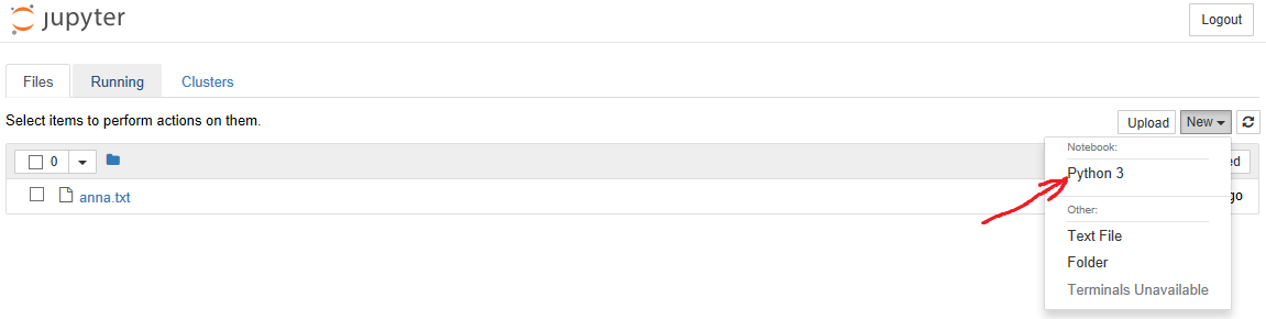
4. The notebook menu opens in the browser, we go there to “New” and select Notebook -> Python 3, as shown in the picture:
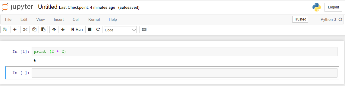
Then the notebook itself opens, where we will drive in the code and admire the result of its work. For example, having driven the code into the “In” cell, we can execute it by pressing Shift + Enter and immediately get the result:
By this time we have dealt with the basic things, now we can proceed to the task itself.
The following is a general recurrent neural network (RNN) architecture that predicts the next symbol (taken from here ):
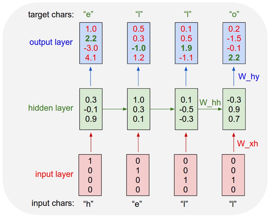
The diagram shows the key feature of RNN - information can be processed cyclically as it moves from input to output, providing (unlike traditional neural networks) a memory effect and allowing processing of related sequences.
Import the necessary libraries:
Load the text of the novel, create a vocabulary of symbols, dictionary objects for translation of the symbol -> code, code -> symbol and encode all the text of the novel (encoded array):
Checking the beginning, the famous phrase in place, everything is in order:
We look, how it looks in the coded form (in this form the data will be processed in the network):
Since our network works with individual characters, we are dealing with a classification problem when we try to predict the next character from the previous text. Dictionary length is essentially the number of classes from which our network will make a choice:
There are a lot of characters in the dictionary, but you need to take into account that upper and lower case letters are different characters, and we also remember a lot of French text, i.e. we actually have two alphabets.
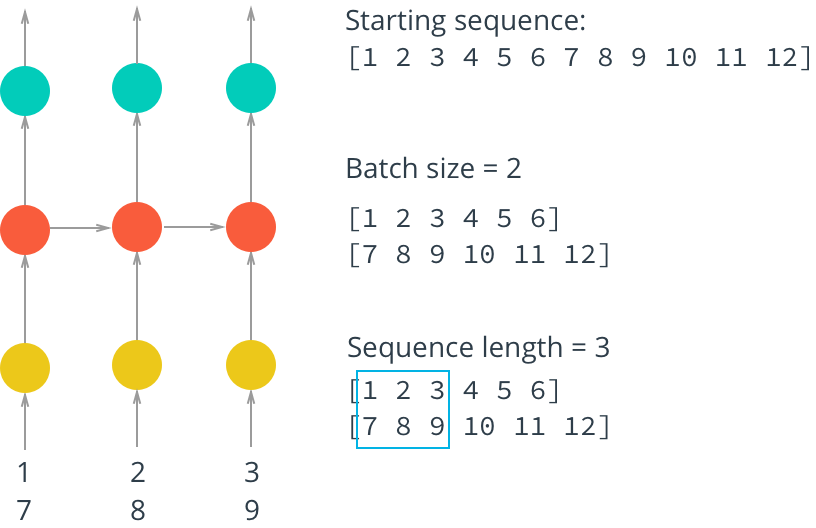
For effective training of our network it is necessary to break the data into packets (mini-batches). First, it saves RAM. If we try to drive all the data into the network at once, the memory may simply not be enough. Secondly, when splitting data into packets, the network will be trained much faster - we can update the weights in the neural network after passing each data packet, as well as parallelize the loading of packets, as shown in the picture:
Create a procedure for obtaining the source packet, which will be fed to the input of the neural network (feature) and the control package, with which the network prediction (target) will be compared:
The function works as a generator , each call to which allows you to get the following pair of "x" and "y", for example:
The output shows a shift of the packet “y” relative to the packet “x”.
Below is a diagram of our RNN model:
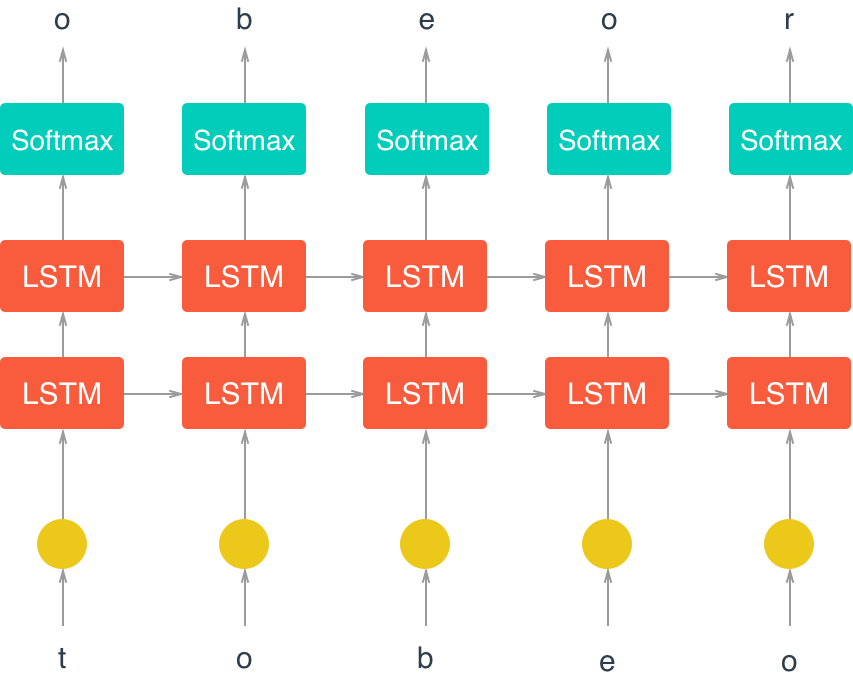
The main learning magic occurs in the LSTM (Long Short Term Memory) cell.
Here is a wonderful article in which the logic of the work of such cells and neural networks based on LSTM is described in simple and understandable English.
When building a model, we first define incoming parameters:
It must be recalled that the data in Tensorflow is stored in tensors .
" placeholders " are the type of tensors that determine the type and format of data (for example, the dimension of the matrix), and the data itself will actually be loaded at the right time in the future.
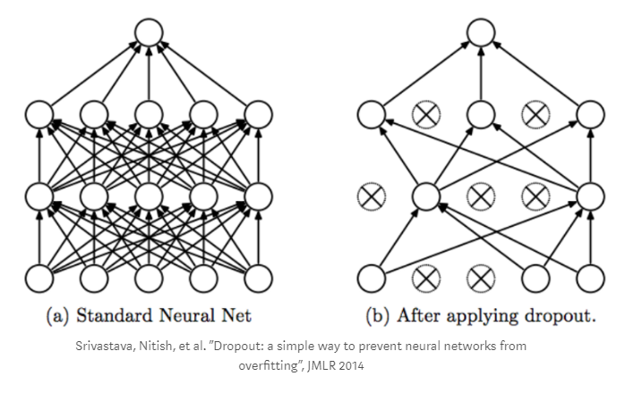
As for drop out, this is a mechanism to counteract the effect of "retraining" our network, when in the process we randomly exclude some of the vertices of our graph from the calculations:
Next we build the structure of the LTSM cell.
Next, we will build the output layer. We are determined with the dimension.
If the input data had the dimension M (batch size), N (sequence length) and passed through hidden layers of size L units, then at the output we get a 3D tensor of dimension MxNxL . To simplify the problem, we make reshape 3D -> 2D and reduce the tensor to the form (M ∗ N) × L. Thus, we will have one line for each sequence and each “step” and the value of each line is the output from LSTM units.
We multiply this matrix by the output level weights matrix and add the output level offset.
At the same time, we initialize the weights with random variables with a truncated normal distribution (in the range of 2 standard deviations), and bias we initialize with zeros, which is a recommended practice in neural networks.
The result of the output layer is passed through the softmax activation function (for more details on the activation functions here ), using the result of this function as a predictor.
Next, we define the loss function (that is, we measure how wrong we are). To do this, we compute softmax cross entropy between the values of the logit function and the label (which in turn are target values that have passed through one-hot encoding).
In deep learning, one-hot coding is often used to represent categorical variables in the form of binary vectors, so that they are more convenient to use in further calculations. For example, the sequence of data:
we can encode in integer (as we did above in the variable encoded) in:
and after one-hot coding it will look like this:
The function of loss in deep learning is considered in different ways. For the tasks of classifying objects that belong to mutually exclusive classes (in our case, the next symbol cannot be both “a” and “b”), the loss function is calculated through the softmax function cross entropy with logits and we return the average value of this function of all elements across all dimensions tensor.
Next, we build an optimizer, which is based on the gradient descent method. In this case, we are protected from two problems (for more details, click here ):
Adam optimizer is used as optimization function.
Now we collect all the details of the puzzle together and build a class that describes our network. The key operator that forms the RNN network is tf.nn.dynamic_rnn. It returns the output of each LSTM cell at each step, for each sequence, in each packet (mini-batch). In addition, it returns the final status of the LSTM cells, which we save and transfer to the input in the first LSTM cell when the next data packet is loaded. At the input of tf.nn.dynamic_rnn, we give the cell (cell), the initial status, which we get from build_lstm and the input data sequence.
Next, we set the hyperparameters for our model. There is a big space for creativity, because by changing these parameters you can “squeeze” more out of the network. I will not dwell on the strategy of setting up, since this is a separate large topic, which is devoted to many articles and studies.
Now we start learning our model.
We launch input and target data into the network, we launch optimization. For each package (mini-batch) we keep the final LSTM status, which we give to the entrance to the network with the next package, ensuring continuity. Periodically (determined by the save_every_n variable) we save the state of our model (with all variables, weights, etc.) in the checkpoint . There is another parameter here - the number of epochs (complete training cycles of the model). It is also necessary to remind that all work with data in Tensorflow is carried out within an open session, which usually begins with the code
Further we observe the learning process:
We see a gradual decrease in training loss.
On my PC, this learning process took about 6 hours. If you have a machine with a good GPU, this period can be reduced by several times.
Check our saved checkpoints:
Now we can proceed to the sampling, that is, to generate text.
The idea is that by feeding one character to the network input, we get the predicted character at the output, which we add to the generated text and feed it again to the network input at the next iteration, etc. The exception is the text for “warming up” of the model, which is fed to the input in the prime parameter.
The
Now we generate the text and see what happened.
To begin with - an early state of the model (after 200 iterations).
On the one hand, it turned out some nonsense. On the other hand, we see that the neural network begins to form an understanding of words as a set of characters, separated by spaces, and even the use of some punctuation marks.
Go ahead (after the 600th iteration).
Here we see and the “words” have become more authentic, some beginnings of dialogues have emerged. At some point, the grid even cursed :)
In general, the positive dynamics is evident.
Well, the result of the last iteration.
Here we see that words are basically composed correctly of letters. Dialogs are marked, punctuation marks are well placed, etc. If you look from afar and do not read the text, it looks decent.
Obviously, our network has not yet learned how to write like Leo Tolstoy, but progress has been made as far as learning is concerned. At the same time, in order to move towards greater meaningfulness, you need to use other methods (for example, word embedding), because with the help of char-wise RNN you can get a good grammar relatively easily, but it’s probably not easy to get meaning from the text.
Nevertheless, this example illustrates what kind of magic can occur within a neural network, despite the fact that no rules, no grammar of the language are given to the input, and it has to be thought of before all this.
Of course, you can submit another text to the input (preferably not less voluminous), in any language, play with hyper parameters and get some other results. I hope that even a simple repetition of the steps described can lead someone to figure out how things work out here and I guarantee that you will have many interesting discoveries along the way :)
In this example, we will construct a recurrent neural network, which, having received the text of Tolstoy’s novel Anna Karenina as an input, will generate its text, somewhat similar to the original, predicting what the next character should be.
The structure of the presentation, I tried to do this so that you can repeat all the steps to a beginner, not even understanding in detail what exactly is happening inside this network. Professionals of Deep Learning most likely will not find here anything interesting, and those who only study these technologies, I ask under kat.
Introduction
The basis of this mini-project were taken articles Andrej Karpathy (links below) and educational materials udacity .
The easiest way to repeat everything described below:
')
- install anaconda distribution with Python 3.6 on your PC
- create a working conda environment
- install tensorflow, numpy, jupyter libraries into this environment
- write and execute code in Jupyter Notebook, which gives us the necessary interactivity
- Download the text of the novel in txt format
In the case of anaconda installation on Windows, do the following:
1. Create a folder in which we will work, copy the text there under the name "anna.txt"
2. Run Anaconda Promt, go to the created folder, create the necessary environment “tolstoy” with the necessary libraries and activate it:
(C:\anaconda3) C:\DL\rnn-tolstoy>conda create -n tolstoy ... (C:\anaconda3) C:\DL\rnn-tolstoy>activate tolstoy (tolstoy) C:\DL\rnn-tolstoy>conda install numpy tensorflow jupyter ... 3. When all libraries are installed, run jupyter notebook, in which we will work:
(tolstoy) C:\DL\rnn-tolstoy>jupyter notebook 4. The notebook menu opens in the browser, we go there to “New” and select Notebook -> Python 3, as shown in the picture:
Then the notebook itself opens, where we will drive in the code and admire the result of its work. For example, having driven the code into the “In” cell, we can execute it by pressing Shift + Enter and immediately get the result:
By this time we have dealt with the basic things, now we can proceed to the task itself.
The following is a general recurrent neural network (RNN) architecture that predicts the next symbol (taken from here ):
The diagram shows the key feature of RNN - information can be processed cyclically as it moves from input to output, providing (unlike traditional neural networks) a memory effect and allowing processing of related sequences.
We initialize and prepare data
Import the necessary libraries:
import time from collections import namedtuple import numpy as np import tensorflow as tf Load the text of the novel, create a vocabulary of symbols, dictionary objects for translation of the symbol -> code, code -> symbol and encode all the text of the novel (encoded array):
with open('anna.txt', 'r') as f: text=f.read() vocab = sorted(set(text)) vocab_to_int = {c: i for i, c in enumerate(vocab)} int_to_vocab = dict(enumerate(vocab)) encoded = np.array([vocab_to_int[c] for c in text], dtype=np.int32) Checking the beginning, the famous phrase in place, everything is in order:
text[:110] Out: ' \n\n\n\nI\n\n , -.' We look, how it looks in the coded form (in this form the data will be processed in the network):
encoded[:110] Out: array([ 99, 77, 93, 94, 102, 1, 91, 82, 92, 79, 77, 105, 0, 0, 0, 0, 30, 0, 0, 79, 123, 111, 1, 123, 129, 106, 123, 124, 117, 114, 108, 133, 111, 1, 123, 111, 118, 134, 114, 1, 121, 120, 127, 120, 112, 114, 1, 110, 122, 125, 109, 1, 119, 106, 1, 110, 122, 125, 109, 106, 7, 1, 116, 106, 112, 110, 106, 137, 1, 119, 111, 123, 129, 106, 123, 124, 117, 114, 108, 106, 137, 1, 123, 111, 118, 134, 137, 1, 119, 111, 123, 129, 106, 123, 124, 117, 114, 108, 106, 1, 121, 120, 8, 123, 108, 120, 111, 118, 125, 9]) Since our network works with individual characters, we are dealing with a classification problem when we try to predict the next character from the previous text. Dictionary length is essentially the number of classes from which our network will make a choice:
len(vocab) Out: 140There are a lot of characters in the dictionary, but you need to take into account that upper and lower case letters are different characters, and we also remember a lot of French text, i.e. we actually have two alphabets.
We divide data into packages
For effective training of our network it is necessary to break the data into packets (mini-batches). First, it saves RAM. If we try to drive all the data into the network at once, the memory may simply not be enough. Secondly, when splitting data into packets, the network will be trained much faster - we can update the weights in the neural network after passing each data packet, as well as parallelize the loading of packets, as shown in the picture:
Create a procedure for obtaining the source packet, which will be fed to the input of the neural network (feature) and the control package, with which the network prediction (target) will be compared:
def get_batches(arr, n_seqs, n_steps): ''' , n_seqs x n_steps arr. --------- arr: , n_seqs: Batch size, n_steps: Sequence length, "" ''' # , characters_per_batch = n_seqs * n_steps n_batches = len(arr)//characters_per_batch # , arr = arr[:n_batches * characters_per_batch] # reshape 1D -> 2D, n_seqs , arr = arr.reshape((n_seqs, -1)) for n in range(0, arr.shape[1], n_steps): # , x = arr[:, n:n+n_steps] # , , "x" y = np.zeros_like(x) y[:, :-1], y[:, -1] = x[:, 1:], x[:, 0] yield x, y The function works as a generator , each call to which allows you to get the following pair of "x" and "y", for example:
batches = get_batches(encoded, 10, 50) x, y = next(batches) print('x\n', x[:5, :5]) print('\ny\n', y[:5, :5]) x [[ 99 77 93 94 102] [ 1 110 108 114 112] [ 79 120 124 1 120] [114 119 1 109 120] [106 108 111 110 117]] y [[ 77 93 94 102 1] [110 108 114 112 111] [120 124 1 120 124] [119 1 109 120 108] [108 111 110 117 114]] The output shows a shift of the packet “y” relative to the packet “x”.
Build a model
Below is a diagram of our RNN model:
The main learning magic occurs in the LSTM (Long Short Term Memory) cell.
Here is a wonderful article in which the logic of the work of such cells and neural networks based on LSTM is described in simple and understandable English.
When building a model, we first define incoming parameters:
def build_inputs(batch_size, num_steps): ''' placeholder' , , drop out --------- batch_size: Batch size, num_steps: Sequence length, "" ''' # placeholder' inputs = tf.placeholder(tf.int32, [batch_size, num_steps], name='inputs') targets = tf.placeholder(tf.int32, [batch_size, num_steps], name='targets') # Placeholder drop out keep_prob = tf.placeholder(tf.float32, name='keep_prob') return inputs, targets, keep_prob It must be recalled that the data in Tensorflow is stored in tensors .
" placeholders " are the type of tensors that determine the type and format of data (for example, the dimension of the matrix), and the data itself will actually be loaded at the right time in the future.
As for drop out, this is a mechanism to counteract the effect of "retraining" our network, when in the process we randomly exclude some of the vertices of our graph from the calculations:
Next we build the structure of the LTSM cell.
def build_lstm(lstm_size, num_layers, batch_size, keep_prob): ''' LSTM . --------- keep_prob: (tf.placeholder) dropout keep probability lstm_size: LSTM num_layers: LSTM batch_size: Batch size ''' ### LSTM def build_cell(lstm_size, keep_prob): # LSTM lstm = tf.contrib.rnn.BasicLSTMCell(lstm_size) # dropout drop = tf.contrib.rnn.DropoutWrapper(lstm, output_keep_prob=keep_prob) return drop # LSTM deep learning cell = tf.contrib.rnn.MultiRNNCell([build_cell(lstm_size, keep_prob) for _ in range(num_layers)]) # LTSM initial_state = cell.zero_state(batch_size, tf.float32) return cell, initial_state Next, we will build the output layer. We are determined with the dimension.
If the input data had the dimension M (batch size), N (sequence length) and passed through hidden layers of size L units, then at the output we get a 3D tensor of dimension MxNxL . To simplify the problem, we make reshape 3D -> 2D and reduce the tensor to the form (M ∗ N) × L. Thus, we will have one line for each sequence and each “step” and the value of each line is the output from LSTM units.
We multiply this matrix by the output level weights matrix and add the output level offset.
At the same time, we initialize the weights with random variables with a truncated normal distribution (in the range of 2 standard deviations), and bias we initialize with zeros, which is a recommended practice in neural networks.
The result of the output layer is passed through the softmax activation function (for more details on the activation functions here ), using the result of this function as a predictor.
def build_output(lstm_output, in_size, out_size): ''' softmax . --------- x: LSTM in_size: , (- LSTM ) out_size: softmax ( ) ''' # , 3D -> 2D seq_output = tf.concat(lstm_output, axis=1) x = tf.reshape(seq_output, [-1, in_size]) # LTSM softmax with tf.variable_scope('softmax'): softmax_w = tf.Variable(tf.truncated_normal((in_size, out_size), stddev=0.1)) softmax_b = tf.Variable(tf.zeros(out_size)) # logit- logits = tf.matmul(x, softmax_w) + softmax_b # softmax out = tf.nn.softmax(logits, name='predictions') return out, logits Next, we define the loss function (that is, we measure how wrong we are). To do this, we compute softmax cross entropy between the values of the logit function and the label (which in turn are target values that have passed through one-hot encoding).
In deep learning, one-hot coding is often used to represent categorical variables in the form of binary vectors, so that they are more convenient to use in further calculations. For example, the sequence of data:
[red, yellow, green]we can encode in integer (as we did above in the variable encoded) in:
[0, 1, 2]and after one-hot coding it will look like this:
[[1, 0, 0],
[0, 1, 0],
[0, 0, 1]]
The function of loss in deep learning is considered in different ways. For the tasks of classifying objects that belong to mutually exclusive classes (in our case, the next symbol cannot be both “a” and “b”), the loss function is calculated through the softmax function cross entropy with logits and we return the average value of this function of all elements across all dimensions tensor.
def build_loss(logits, targets, lstm_size, num_classes): ''' logit- . --------- logits: logit- targets: , lstm_size: LSTM num_classes: ( ) ''' # one-hot logits y_one_hot = tf.one_hot(targets, num_classes) y_reshaped = tf.reshape(y_one_hot, logits.get_shape()) # softmax cross entropy loss loss = tf.nn.softmax_cross_entropy_with_logits(logits=logits, labels=y_reshaped) loss = tf.reduce_mean(loss) return loss Next, we build an optimizer, which is based on the gradient descent method. In this case, we are protected from two problems (for more details, click here ):
- "Disappearance" of the gradient (protection is built into the logic of the LSTM cells);
- Gradient “explosion” (for this we use gradient clipping here).
Adam optimizer is used as optimization function.
def build_optimizer(loss, learning_rate, grad_clip): ''' , . Arguments: loss: learning_rate: ''' # , "" tvars = tf.trainable_variables() grads, _ = tf.clip_by_global_norm(tf.gradients(loss, tvars), grad_clip) train_op = tf.train.AdamOptimizer(learning_rate) optimizer = train_op.apply_gradients(zip(grads, tvars)) return optimizer Now we collect all the details of the puzzle together and build a class that describes our network. The key operator that forms the RNN network is tf.nn.dynamic_rnn. It returns the output of each LSTM cell at each step, for each sequence, in each packet (mini-batch). In addition, it returns the final status of the LSTM cells, which we save and transfer to the input in the first LSTM cell when the next data packet is loaded. At the input of tf.nn.dynamic_rnn, we give the cell (cell), the initial status, which we get from build_lstm and the input data sequence.
class CharRNN: def __init__(self, num_classes, batch_size=64, num_steps=50, lstm_size=128, num_layers=2, learning_rate=0.001, grad_clip=5, sampling=False): # ( ), # if sampling == True: batch_size, num_steps = 1, 1 else: batch_size, num_steps = batch_size, num_steps tf.reset_default_graph() # input placeholder' self.inputs, self.targets, self.keep_prob = build_inputs(batch_size, num_steps) # LSTM cell, self.initial_state = build_lstm(lstm_size, num_layers, batch_size, self.keep_prob) ### RNN # one-hot x_one_hot = tf.one_hot(self.inputs, num_classes) # RNN outputs, state = tf.nn.dynamic_rnn(cell, x_one_hot, initial_state=self.initial_state) self.final_state = state # (softmax) logit- self.prediction, self.logits = build_output(outputs, lstm_size, num_classes) # ( ) self.loss = build_loss(self.logits, self.targets, lstm_size, num_classes) self.optimizer = build_optimizer(self.loss, learning_rate, grad_clip) We select hyper parameters
Next, we set the hyperparameters for our model. There is a big space for creativity, because by changing these parameters you can “squeeze” more out of the network. I will not dwell on the strategy of setting up, since this is a separate large topic, which is devoted to many articles and studies.
batch_size = 100 # num_steps = 100 # lstm_size = 512 # LSTM num_layers = 2 # LSTM learning_rate = 0.001 # keep_prob = 0.5 # Dropout keep probability We teach the model
Now we start learning our model.
We launch input and target data into the network, we launch optimization. For each package (mini-batch) we keep the final LSTM status, which we give to the entrance to the network with the next package, ensuring continuity. Periodically (determined by the save_every_n variable) we save the state of our model (with all variables, weights, etc.) in the checkpoint . There is another parameter here - the number of epochs (complete training cycles of the model). It is also necessary to remind that all work with data in Tensorflow is carried out within an open session, which usually begins with the code
with tf.Session() as sess: epochs = 20 # N save_every_n = 200 model = CharRNN(len(vocab), batch_size=batch_size, num_steps=num_steps, lstm_size=lstm_size, num_layers=num_layers, learning_rate=learning_rate) saver = tf.train.Saver(max_to_keep=100) with tf.Session() as sess: sess.run(tf.global_variables_initializer()) # checkpoint' #saver.restore(sess, 'checkpoints/______.ckpt') counter = 0 for e in range(epochs): # new_state = sess.run(model.initial_state) loss = 0 for x, y in get_batches(encoded, batch_size, num_steps): counter += 1 start = time.time() feed = {model.inputs: x, model.targets: y, model.keep_prob: keep_prob, model.initial_state: new_state} batch_loss, new_state, _ = sess.run([model.loss, model.final_state, model.optimizer], feed_dict=feed) end = time.time() print('Epoch: {}/{}... '.format(e+1, epochs), 'Training Step: {}... '.format(counter), 'Training loss: {:.4f}... '.format(batch_loss), '{:.4f} sec/batch'.format((end-start))) if (counter % save_every_n == 0): saver.save(sess, "checkpoints/i{}_l{}.ckpt".format(counter, lstm_size)) saver.save(sess, "checkpoints/i{}_l{}.ckpt".format(counter, lstm_size)) Further we observe the learning process:
Epoch: 1/20... Training Step: 1... Training loss: 4.9402... 7.7964 sec/batch Epoch: 1/20... Training Step: 2... Training loss: 4.8530... 7.1318 sec/batch ... Epoch: 20/20... Training Step: 3400... Training loss: 1.4003... 6.6569 sec/batch We see a gradual decrease in training loss.
On my PC, this learning process took about 6 hours. If you have a machine with a good GPU, this period can be reduced by several times.
Check our saved checkpoints:
tf.train.get_checkpoint_state('checkpoints') model_checkpoint_path: "checkpoints\\i3400_l512.ckpt" all_model_checkpoint_paths: "checkpoints\\i200_l512.ckpt" all_model_checkpoint_paths: "checkpoints\\i400_l512.ckpt" all_model_checkpoint_paths: "checkpoints\\i600_l512.ckpt" all_model_checkpoint_paths: "checkpoints\\i800_l512.ckpt" all_model_checkpoint_paths: "checkpoints\\i1000_l512.ckpt" all_model_checkpoint_paths: "checkpoints\\i1200_l512.ckpt" all_model_checkpoint_paths: "checkpoints\\i1400_l512.ckpt" all_model_checkpoint_paths: "checkpoints\\i1600_l512.ckpt" all_model_checkpoint_paths: "checkpoints\\i1800_l512.ckpt" all_model_checkpoint_paths: "checkpoints\\i2000_l512.ckpt" all_model_checkpoint_paths: "checkpoints\\i2200_l512.ckpt" all_model_checkpoint_paths: "checkpoints\\i2400_l512.ckpt" all_model_checkpoint_paths: "checkpoints\\i2600_l512.ckpt" all_model_checkpoint_paths: "checkpoints\\i2800_l512.ckpt" all_model_checkpoint_paths: "checkpoints\\i3000_l512.ckpt" all_model_checkpoint_paths: "checkpoints\\i3200_l512.ckpt" all_model_checkpoint_paths: "checkpoints\\i3400_l512.ckpt" Generate text
Now we can proceed to the sampling, that is, to generate text.
The idea is that by feeding one character to the network input, we get the predicted character at the output, which we add to the generated text and feed it again to the network input at the next iteration, etc. The exception is the text for “warming up” of the model, which is fed to the input in the prime parameter.
The
pick_top_n function pick_top_n used to reduce the “noise” of predictions, leaving only a specified number (default 5) of options for selection, discarding all other options. def pick_top_n(preds, vocab_size, top_n=5): p = np.squeeze(preds) p[np.argsort(p)[:-top_n]] = 0 p = p / np.sum(p) c = np.random.choice(vocab_size, 1, p=p)[0] return c def sample(checkpoint, n_samples, lstm_size, vocab_size, prime=" ."): samples = [c for c in prime] model = CharRNN(len(vocab), lstm_size=lstm_size, sampling=True) saver = tf.train.Saver() with tf.Session() as sess: saver.restore(sess, checkpoint) new_state = sess.run(model.initial_state) for c in prime: x = np.zeros((1, 1)) x[0,0] = vocab_to_int[c] feed = {model.inputs: x, model.keep_prob: 1., model.initial_state: new_state} preds, new_state = sess.run([model.prediction, model.final_state], feed_dict=feed) c = pick_top_n(preds, len(vocab)) samples.append(int_to_vocab[c]) for i in range(n_samples): x[0,0] = c feed = {model.inputs: x, model.keep_prob: 1., model.initial_state: new_state} preds, new_state = sess.run([model.prediction, model.final_state], feed_dict=feed) c = pick_top_n(preds, len(vocab)) samples.append(int_to_vocab[c]) return ''.join(samples) Now we generate the text and see what happened.
To begin with - an early state of the model (after 200 iterations).
checkpoint = 'checkpoints/i200_l512.ckpt' samp = sample(checkpoint, 1000, lstm_size, len(vocab)) print(samp) INFO:tensorflow:Restoring parameters from checkpoints/i200_l512.ckpt . – ,, , , , , , , , , , , , ,.. – , , , , On the one hand, it turned out some nonsense. On the other hand, we see that the neural network begins to form an understanding of words as a set of characters, separated by spaces, and even the use of some punctuation marks.
Go ahead (after the 600th iteration).
checkpoint = 'checkpoints/i600_l512.ckpt' samp = sample(checkpoint, 1000, lstm_size, len(vocab)) print(samp) INFO:tensorflow:Restoring parameters from checkpoints/i600_l512.ckpt . , , , - , , , , , . – , , . , – . – , , , , , , , , , Here we see and the “words” have become more authentic, some beginnings of dialogues have emerged. At some point, the grid even cursed :)
In general, the positive dynamics is evident.
Well, the result of the last iteration.
checkpoint = tf.train.latest_checkpoint('checkpoints') samp = sample(checkpoint, 2000, lstm_size, len(vocab)) print(samp) INFO:tensorflow:Restoring parameters from checkpoints\i3400_l512.ckpt . , , , , . . , , . – , , – , – , - , , , , , , . . , , , . – . , , , . – , , – . – , , , . , , . , – . – . – , , – , – , , – . – , , – , – , , , , – , , – . «, , . , , , – , , , – - . – , . . , – , . , Here we see that words are basically composed correctly of letters. Dialogs are marked, punctuation marks are well placed, etc. If you look from afar and do not read the text, it looks decent.
Conclusion
Obviously, our network has not yet learned how to write like Leo Tolstoy, but progress has been made as far as learning is concerned. At the same time, in order to move towards greater meaningfulness, you need to use other methods (for example, word embedding), because with the help of char-wise RNN you can get a good grammar relatively easily, but it’s probably not easy to get meaning from the text.
Nevertheless, this example illustrates what kind of magic can occur within a neural network, despite the fact that no rules, no grammar of the language are given to the input, and it has to be thought of before all this.
Of course, you can submit another text to the input (preferably not less voluminous), in any language, play with hyper parameters and get some other results. I hope that even a simple repetition of the steps described can lead someone to figure out how things work out here and I guarantee that you will have many interesting discoveries along the way :)
Source: https://habr.com/ru/post/342738/
All Articles