The first part of the article can be proof that ray tracing is an elegant example of software that allows you to create stunningly beautiful images using only simple and intuitive algorithms.

Unfortunately, this simplicity comes at a price: poor performance. Despite the fact that there are many ways to optimize and parallelize ray tracer, they still remain too costly from the point of view of calculations to perform in real time; and although the equipment continues to evolve and becomes faster every year, in some areas of use beautiful, but hundreds of times faster images are needed today . Of all these areas of application, the most demanding are games: we expect to render excellent pictures at a frequency of at least 60 frames per second. Ray tracers simply can't handle it.
')
Then how is the game doing?

The answer is to use a completely different family of algorithms, which we explore in the second part of the article. Unlike ray tracing, which was obtained from simple geometric models of image formation in the human eye or in the camera, now we will start from the other end - we will ask ourselves what we can draw on the screen and how to draw it as quickly as possible. As a result, we get completely different algorithms that create roughly similar results.

Straight lines

Let's start from scratch again: we have a canvas with dimensions $$$C_w$ and $$$C_h$ and we can put a pixel on it ( $$$PutPixel ()$ ).

Let's say we have two points $$$P_0$ and $$$P_1$ with coordinates $$$(x_0, y_0)$ and $$$(x_1, y_1)$ . Drawing these two points separately is trivial; but how can you draw a straight line segment from $$$P_0$ at $$$P_1$ ?

Let's start with the representation of the line with parametric coordinates, as we did before with the rays (these “rays” are nothing but lines in 3D). Any point on the line can be obtained by starting with $$$P_0$ and moving some distance away from $$$P_0$ to $$$P_1$ :

$$

$$P = P_0 + t (P_1 - P_0)$$

We can decompose this equation into two, one for each of the coordinates:

$$

$$x = x_0 + t (x_1 - x_0)$$

$$

$$y = y_0 + t (y_1 - y_0)$$

Let's take the first equation and calculate $$$t$ :

$$

$$x = x_0 + t (x_1 - x_0)$$

$$

$$x - x_0 = t (x_1 - x_0)$$

$$

$${{x - x_0} \ over {x_1 - x_0}} = t$$

Now we can substitute this expression in the second equation instead of $$$t$ :

$$

$$y = y_0 + t (y_1 - y_0)$$

$$

$$y = y_0 + {{x - x_0} \ over {x_1 - x_0}} (y_1 - y_0)$$

Let's transform it a bit:

$$

$$y = y_0 + (x - x_0) {{y_1 - y_0} \ over {x_1 - x_0}}$$

Notice that $$${{y_1 - y_0} \ over {x_1 - x_0}}$ Is a constant that depends only on the end points of the segment; let's label it $$$a$ :

$$

$$y = y_0 + a (x - x_0)$$

What is $$$a$ ? Judging by how it is defined, it is an indicator of a change in the coordinates $$$y$ to change the unit of length coordinates $$$x$ ; in other words, it is an indicator of the slope of a straight line.

Let's go back to the equation. Open brackets:

$$

$$y = y_0 + ax - ax_0$$

Group constants:

$$

$$y = ax + (y_0 - ax_0)$$

Expression $$$(y_0 - ax_0)$ depends again only on the end points of the segment; let's label it $$$b$ and finally get

$$

$$y = ax + b$$

This is a classic linear function with which almost all lines can be represented. It cannot describe vertical straight lines, because they have an infinite number of values. $$$y$ at one value $$$x$ and none for all the others. Sometimes in the process of obtaining such a representation from the original parametric equation, such families of lines can be missed; this happens when calculating $$$t$ because we ignored what $$$x_1 - x_0$ can give division by zero. For now let's just ignore the vertical lines; we will get rid of this restriction later.

So now we have a way to calculate the value. $$$y$ for any value we are interested in $$$x$ . In this case, we get a couple $$$(x, y)$ satisfying the equation of a line. If we move from $$$x_0$ to $$$x_1$ and calculate the value $$$y$ for each value $$$x$ Then we get the first approximation of our line drawing function:

DrawLine(P0, P1, color) { a = (y1 - y0)/(x1 - x0) b = y0 - a*x0 for x = x0 to x1 { y = a*x + b canvas.PutPixel(x, y, color) } } 

In this fragment, x0 and y0 are the coordinates. $$$x$ and $$$y$ points P0 ; I will use this convenient entry in the future. Also note that the division operator / should not do integer division, but division of real numbers.

This function is a direct naive interpretation of the above equation, so it is obvious that it works; but can we speed up her work?

Note that we do not calculate values. $$$y$ for all $$$x$ : in fact, we only compute them as integer increments $$$x$ and we do it in the following order: immediately after the calculation $$$y (x)$ we calculate $$$y (x + 1)$ :

$$

$$y (x) = ax + b$$

$$

$$y (x + 1) = a (x + 1) + b$$

We can use this to create a faster algorithm. Let's take the difference between $$$y$ consecutive pixels:

$$

$$y (x + 1) - y (x) = (a (x + 1) + b) - (ax + b)$$

$$

$$= a (x + 1) + b - ax - b$$

$$

$$= ax + a - ax$$

$$

$$= a$$

This is not very surprising; after all the slope $$$a$ - is an indicator of how $$$y$ changes per increment unit $$$x$ that is exactly what we are doing here.

Interestingly, we can obtain the following in a trivial way:

$$

$$y (x + 1) = y (x) + a$$

This means that we can calculate the following value. $$$y$ only using the previous value $$$y$ and the addition of slope; per-pixel multiplication is not required. We need to start somewhere (at the very beginning there is no "previous value $$$y$ "So we will start with $$$(x_0, y_0)$ and then we will add $$$1$ to $$$x$ and $$$a$ to $$$y$ until we get to $$$x_0$ .

Considering that $$$x_0 <x_1$ , we can rewrite the function as follows:

 DrawLine(P0, P1, color) { a = (y1 - y0)/(x1 - x0) y = y0 for x = x0 to x1 { canvas.PutPixel(x, y, color) y = y + a } } 

This new version of the function has a new limitation: it can only draw straight lines from left to right, that is, when $$$x_0 <x_1$ . This problem is quite easy to get around: since it doesn't matter in which order we draw individual pixels, if we have a straight line from right to left, we simply change P0 and P1 to turn it into a left-right version of the same straight line, then draw it as earlier:

 DrawLine(P0, P1, color) { # Make sure x0 < x1 if x0 > x1 { swap(P0, P1) } a = (y1 - y0)/(x1 - x0) y = y0 for x = x0 to x1 { canvas.PutPixel(x, y, color) y = y + a } } 

Now we can draw a pair of lines. Here is $$$(- 200, 100) - (240, 120)$ :



Here is how it looks close:



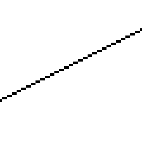
The straight line looks like a broken line, because we can draw pixels only on integer coordinates, and the mathematical straight lines actually have zero width; the picture we draw is a discretized approximation to the ideal straight line $$$(- 200, 100) - (240, 120)$ (Note: there are ways of drawing more beautiful approximate straight lines. We will not use for two reasons: 1) it is slower, 2) our goal is not to draw beautiful straight lines, but to develop basic algorithms for rendering 3D scenes.).

Let's try to draw another straight line, $$$(- 50, -200) - (60, 240)$ :



And here is how it looks close:



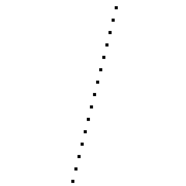
Oh. What happened?

The algorithm worked as intended; he went from left to right, calculated the value $$$y$ for each value $$$x$ and drawn the corresponding pixel. The problem is that he calculated one value $$$y$ for each value $$$x$ , while for some values $$$x$ we need several values $$$y$ .

This is a direct consequence of the choice of the formulation in which $$$y = f (x)$ ; in fact, for the same reason, we cannot draw vertical lines, a limiting case in which there is one value $$$x$ with multiple meanings $$$y$ .

We can draw horizontal lines without any problems. Why are we not able to draw vertical lines just as easily?

As it turns out, we can do it. Selection $$$y = f (x)$ was an arbitrary decision, so there is no reason why it’s difficult to express directly as $$$x = f (y)$ by reworking all the equations and changing $$$x$ and $$$y$ to get the following algorithm as a result:

 DrawLine(P0, P1, color) { # Make sure y0 < y1 if y0 > y1 { swap(P0, P1) } a = (x1 - x0)/(y1 - y0) x = x0 for y = y0 to y1 { canvas.PutPixel(x, y, color) x = x + a } } 

This is similar to the previous DrawLine , with the exception of changing the places of calculations $$$x$ and $$$y$ . The resulting function can handle vertical lines and can correctly draw $$$(0, 0) - (50, 100)$ ; Of course, it will not cope with horizontal lines and will not be able to draw correctly. $$$(0, 0) - (100, 50)$ ! What do we do?

We just need to choose the right version of the function, depending on the line that needs to be drawn. And the criteria will be fairly simple; does direct have more distinct meanings $$$x$ or $$$y$ ? If there are more values $$$x$ than $$$y$ , we use the first version; otherwise, the second is applied.

Here is the DrawLine version that handles all cases:

 DrawLine(P0, P1, color) { dx = x1 - x0 dy = y1 - y0 if abs(dx) > abs(dy) { #     # ,  x0 < x1 if x0 > x1 { swap(P0, P1) } a = dy/dx y = y0 for x = x0 to x1 { canvas.PutPixel(x, y, color) y = y + a } } else { #     # ,  y0 < y1 if y0 > y1 { swap(P0, P1) } a = dx/dy x = x0 for y = y0 to y1 { canvas.PutPixel(x, y, color) x = x + a } } } 

This will certainly work, but the code is not very beautiful; there are two code implementations that incrementally calculate a linear function, and this logic of computation and selection is mixed. Since we will often use linear functions, it is worth spending a little time to separate the code.

We have two functions $$$y = f (x)$ and $$$x = f (y)$ . To abstract from the fact that we work with pixels, let's write this in a general form as $$$d = f (i)$ where $$$i$ - an independent variable for which we select values, and $$$d$ - dependent variable whose values ​​depend on another, and which we want to calculate. In case of more horizontal straight $$$x$ is an independent variable as well $$$y$ - dependent; in the case of a more vertical line, the opposite is true.

Of course, any function can be written as $$$d = f (i)$ . We know two more aspects that completely define it: its linearity and its two values; namely, $$$d_0 = f (i_0)$ and $$$d_1 = f (i_1)$ . We can write a simple method that gets these values ​​and returns intermediate values. $$$d$ , believing, as before, that $$$i1 <i0$ :

 Interpolate (i0, d0, i1, d1) { values = [] a = (d1 - d0) / (i1 - i0) d = d0 for i = i0 to i1 { values.append(d) d = d + a } return values } 

Notice that value $$$d$ corresponding to $$$i_0$ , is in values[0] , value for $$$i_0 + 1$ is in values[1] , and so on; generally meaning $$$i_n$ is in values[i_n - i_0] , if we assume that $$$i_n$ is in the interval $$$[i_0, i_1]$ .

There is a dead-end case to consider; we may need to calculate $$$d = f (i)$ for single meaning $$$i$ that is, when $$$i0 = i1$ . In this case, we cannot even calculate $$$a$ , so we will handle this as a special case:

 Interpolate (i0, d0, i1, d1) { if i0 == i1 { return [ d0 ] } values = [] a = (d1 - d0) / (i1 - i0) d = d0 for i = i0 to i1 { values.append(d) d = d + a } return values } 

Now we can write DrawLine using Interpolate :

 DrawLine(P0, P1, color) { if abs(x1 - x0) > abs(y1 - y0) { #     # ,  x0 < x1 if x0 > x1 { swap(P0, P1) } ys = Interpolate(x0, y0, x1, y1) for x = x0 to x1 { canvas.PutPixel(x, ys[x - x0], color) } } else { #     # ,  y0 < y1 if y0 > y1 { swap(P0, P1) } xs = Interpolate(y0, x0, y1, x1) for y = y0 to y1 { canvas.PutPixel(xs[y - y0], y, color) } } } 

This DrawLine can handle all cases correctly:



Source code and working demo >>

Although this version is not much shorter than the previous one, it clearly shares the calculation of intermediate values $$$y$ and $$$x$ , the decision on the choice of an independent variable plus the drawing code itself. The advantage of this is perhaps not entirely obvious, but we will actively use Interpolate again in subsequent chapters.

Note that this is not the best or fastest rendering algorithm; Interpolate , not DrawLine an important result of this chapter. The best algorithm for drawing lines is most likely the Brezenham algorithm.

Filled triangles

We can use the DrawLine method to draw the outline of a triangle. This type of contour is called a frame , because it looks like a triangle frame:

 DrawWireframeTriangle (P0, P1, P2, color) { DrawLine(P0, P1, color); DrawLine(P1, P2, color); DrawLine(P2, P0, color); } 

We get the following result:



Can we fill the triangle with some color?

As usually happens in computer graphics, for this there are many ways. We will draw the filled triangles, perceiving them as a set of segments of horizontal lines, which, if drawn together, look like a triangle. Below is a very rough first approximation of what we want to do:

    y  ,    x_left  x_right   y DrawLine(x_left, y, x_right, y) 

Let's start with the “for each y coordinate a horizontal line occupied by a triangle”. The triangle is defined by three vertices. $$$P_0$ , $$$P_1$ and $$$P_2$ . If we sort these points by increasing the value $$$y$ , so that $$$y_0 \ le y_1 \ le y_2$ , the value range $$$y$ occupied by a triangle will be equal to $$$[y_0, y_2]$ :

 if y1 < y0 { swap(P1, P0) } if y2 < y0 { swap(P2, P0) } if y2 < y1 { swap(P2, P1) } 

Then we need to calculate x_left and x_right . This is a little more difficult, because the triangle has three, not two sides. However in terms of the values $$$y$ we always have a “long” side from $$$P_0$ before $$$P_2$ and two “short” sides from $$$P_0$ before $$$P_1$ and from $$$P_1$ lj $$$P_2$ (Note: there is a special case where $$$y_0 = y_1$ or $$$y_1 = y_2$ , that is, when the triangle has a horizontal side; in such cases there are two sides that can be considered “long” sides. Fortunately, it does not matter which side we choose, so we can stick to this definition.). That is, the x_right values x_right obtained either from the long side, or from both short sides; and x_left values x_left obtained from another set.

We'll start by calculating the values. $$$x$ for three sides. Since we draw horizontal lines, we need exactly one value. $$$x$ for each value $$$y$ ; this means that we can get the values ​​directly using Interpolate , using as an independent value $$$y$ , and as a dependent value $$$x$ :

 x01 = Interpolate(y0, x0, y1, x1) x12 = Interpolate(y1, x1, y2, x2) x02 = Interpolate(y0, x0, y2, x2) 

x02 will be either x_left or x_right ; the other is the concatenation of x01 and x12 .

Notice that in these two lists there is a duplicate value: the value $$$x$ for $$$y_1$ is the last value of x01 , and the first value of x12 . We just need to get rid of one of them.

 remove_last(x01) x012 = x01 + x12 

Finally, we have x02 and x012 , and we need to determine which of them is x_left and x_right . To do this, look at the values. $$$x$ for one of the lines, for example, for the average:

 m = x02.length / 2 if x02[m] < x012[m] { x_left = x02 x_right = x012 } else { x_left = x012 x_right = x02 } 

Now it only remains to draw horizontal lines. For reasons that will become clear later, we will not use DrawLine for this; instead, we will draw the pixels separately.

Here is the full version of DrawFilledTriangle :

 DrawFilledTriangle (P0, P1, P2, color) { #   ,  y0 <= y1 <= y2 if y1 < y0 { swap(P1, P0) } if y2 < y0 { swap(P2, P0) } if y2 < y1 { swap(P2, P1) } #   x   x01 = Interpolate(y0, x0, y1, x1) x12 = Interpolate(y1, x1, y2, x2) x02 = Interpolate(y0, x0, y2, x2) #    remove_last(x01) x012 = x01 + x12 # ,       m = x012.length / 2 if x02[m] < x012[m] { x_left = x02 x_right = x012 } else { x_left = x012 x_right = x02 } #    for y = y0 to y2 { for x = x_left[y - y0] to x_right[y - y0] { canvas.PutPixel(x, y, color) } } } 

Here is the result; to check we called DrawFilledTriangle , and then DrawWireframeTriangle with the same coordinates, but in different colors: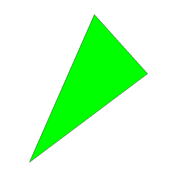



Source code and working demo >>

You may notice that the black outline of the triangle does not completely coincide with the green inner region; this is especially noticeable in the lower right edge of the triangle. This is because DrawLine () computes $$$y = f (x)$ for this edge, but DrawTriangle () computes $$$x = f (y)$ . We are ready to go for such an approximation in order to achieve our goal - high-speed rendering.

Shaded Triangles

In the previous section, we developed an algorithm for drawing a triangle and filling it with color. Our next goal will be to draw a shaded triangle that looks like a gradient-filled one.

Although shaded triangles look prettier than monochrome, this is not the main purpose of the chapter; this is just a special application of the technique we will create. It will probably be the most important in this section of the article; almost everything else will be built on its basis.

But let's start with the simple. Instead of filling the triangle with a solid color, we want to fill it with shades of color. It will look like this:



Source code and working demo >>

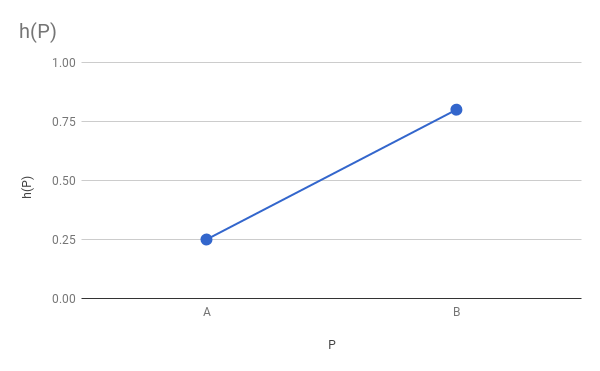
The first step is to formally define what we want to draw. To do this, we will assign a real value to each vertex. $$$h$ denoting the brightness of the vertex color. $$$h$ is in the interval $$$[0.0, 1.0]$ .

To get the exact color of a pixel, having a color $$$C$ and brightness $$$h$ , we just do per channel multiplication: $$$C_h = (R_C * h, G_C * h, B_C * h)$ . That is, when $$$h = 0.0$ we get black, and when $$$h = 1.0$ - original color $$$C$ .

Edge Shading Calculation

So, to draw a shaded triangle, we need to calculate the value $$$h$ for each pixel of the triangle, get the appropriate shade of color and color the pixel Everything is very simple!

However, at this stage we only know the values $$$h$ for given vertices. How to calculate values $$$h$ for the rest of the triangle?

Let's first look at the edges. Choose edge $$$Ab$ . We know $$$h_A$ and $$$h_B$ . What happens in $$$M$ that is, in the middle of the segment $$$Ab$ ? Since we want the brightness to change smoothly from $$$A$ to $$$B$ then $$$h_M$ there must be some value between $$$h_A$ and $$$h_B$ . Because $$$M$ Is the midpoint of the segment $$$Ab$ then why not do $$$h_M$ average value $$$h_A$ and $$$h_B$ ?

If more formally, then we have a function $$$h = f (P)$ for which we know the limit values $$$h (A)$ and $$$h (B)$ and we need to make it smooth. We don't know anything more about $$$h = f (P)$ Therefore, we can choose any function that meets these criteria, for example, a linear function:



Of course, the basis of the shaded triangle code will be the solid triangle code created in the previous chapter. One of their first steps involves calculating the end points of each horizontal line, i.e. x_left and x_right for the sides $$$P_0P_1$ , $$$P_0P_2$ and $$$P_1P_2$ ; we used Interpolate() to calculate values $$$x = f (y)$ , having $$$x (y_0)$ and $$$x (y_1)$ ... and that is exactly what we want to do here; it is enough to replace $$$x$ on $$$h$ !

That is, we can calculate intermediate values $$$h$ in exactly the same way as we calculated the values $$$x$ :

 x01 = Interpolate(y0, x0, y1, x1) h01 = Interpolate(y0, h0, y1, h1) x12 = Interpolate(y1, x1, y2, x2) h12 = Interpolate(y1, h1, y2, h2) x02 = Interpolate(y0, x0, y2, x2) h02 = Interpolate(y0, h0, y2, h2) 

The next step will be the transformation of these three vectors into two vectors and the determination of which of them represents left-sided values ​​and which of them represents right-sided values. Note that the values $$$h$ play no role in what they are; it is completely determined by the values $$$x$ . Meanings $$$h$ "Stick" to the values $$$x$ , because they are other attributes of the same physical pixels. That is, if x012 has values ​​for the right side of the triangle, then h012 has values ​​for the right side of the triangle:

  #    remove_last(x01) x012 = x01 + x12 remove_last(h01) h012 = h01 + h12 # ,       m = x012.length / 2 if x02[m] < x012[m] { x_left = x02 x_right = x012 h_left = h02 h_right = h012 } else { x_left = x012 x_right = x02 h_left = h012 h_right = h02 } 

Internal shading calculation

The only step left is to draw the horizontal segments themselves. For each segment we know $$$x_ {left}$ and $$$x_ {right}$ and now we also know $$$h_ {left}$ and $$$h_ {right}$ . However, instead of iterating from left to right and drawing each pixel with the base color, we need to calculate the values $$$h$ for each pixel of the segment.

We can again assume that $$$h$ varies linearly with $$$x$ and use Interpolate() to calculate these values:

 h_segment = Interpolate(x_left[y-y0], h_left[y-y0], x_right[y-y0], h_right[y-y0]) 

And now it's just a matter of calculating the color for each pixel and drawing it.

Here is the calculation code for DrawShadedTriangle :

 DrawShadedTriangle (P0, P1, P2, color) { #   ,  y0 <= y1 <= y2 if y1 < y0 { swap(P1, P0) } if y2 < y0 { swap(P2, P0) } if y2 < y1 { swap(P2, P1) } #   x   h    x01 = Interpolate(y0, x0, y1, x1) h01 = Interpolate(y0, h0, y1, h1) x12 = Interpolate(y1, x1, y2, x2) h12 = Interpolate(y1, h1, y2, h2) x02 = Interpolate(y0, x0, y2, x2) h02 = Interpolate(y0, h0, y2, h2) #    remove_last(x01) x012 = x01 + x12 remove_last(h01) h012 = h01 + h12 # ,       m = x012.length / 2 if x02[m] < x012[m] { x_left = x02 x_right = x012 h_left = h02 h_right = h012 } else { x_left = x012 x_right = x02 h_left = h012 h_right = h02 } #    for y = y0 to y2 { x_l = x_left[y - y0] x_r = x_right[y - y0] h_segment = Interpolate(x_l, h_left[y - y0], x_r, h_right[y - y0]) for x = x_l to x_r { shaded_color = color*h_segment[x - xl] canvas.PutPixel(x, y, shaded_color) } } } 

This algorithm is much more general than it may seem: until the moment in which $$$h$ multiplied by color then what $$$h$ is the brightness of color, does not play any role. This means that we can use this technique to calculate the value of anything that can be represented as a real number for each pixel of a triangle, starting with the values ​​of this property at the vertices of the triangle and considering that the property changes linearly on the screen.

Therefore, this algorithm will prove invaluable in the subsequent parts; do not continue reading until you are sure you understand it well.

Perspective Projection

For a while, we leave 2D-triangles alone and pay attention to 3D; and more specifically, on how to represent 3D objects on a 2D surface.

In the same way as we did at the beginning of the ray tracing part, we will start by specifying the camera . We use the same conditions: the camera is in $$$O = (0, 0, 0)$ looking in the direction $$$\ vec {Z _ +}$ and the “up” vector is $$$\ vec {Y _ +}$ . We will also define a rectangular viewport with a size $$$V_w$ on $$$V_h$ whose edges are parallel $$$\ vec {X}$ and $$$\ vec {Y}$ and being at a distance $$$d$ from the camera. If any of this is incomprehensible to you, read the chapter Basics of ray tracing .

Consider the point $$$P$ somewhere in front of the camera. The camera "sees" $$$P$ , that is, there is a certain ray of light reflected from $$$P$ and reaching the camera. We are interested in finding the point $$$P '$ in which the light beam crosses the viewing window (note that this is the opposite of our actions in ray tracing when we started from a point in the viewing window and determined what is visible through it):



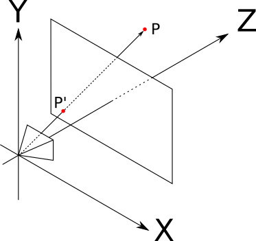
Here is a diagram of the situation, visible "right", that is, when $$$\ vec {Y _ +}$ pointing up $$$\ vec {Z _ +}$ pointing right as well $$$\ vec {X _ +}$ sent to us:



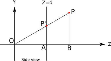
In addition to $$$O$ , $$$P$ and $$$P '$ this diagram shows points $$$A$ and $$$B$ which will be useful for understanding the situation.

It is clear that $$$P'_Z = d$ because we have determined that $$$P '$ Is a point in the viewport, and the viewport is located on the plane $$$Z = d$ .

It should also be clear that the triangles $$$OP'A$ and $$$OPB$ similar: they have two common sides $$$OA$ similar to $$$OB$ and $$$OP$ similar to $$$OP '$ ) and their remaining sides are parallel ( $$$P'A$ and $$$PB$ ). This implies that the following equation of proportionality holds:

$$

$${| P'A | \ over | OA |} = {| PB | \ over | OB |}$$

From it we get

$$

$$|P'A| = {|PB| \cdot |OA| \over {|OB|}}$$

The length of each segment (with a sign) in this equation is the coordinate of the point that we know or that we need: $$$|P'A| = P'_Y$ , $$$|PB| = P_Y$ , $$$|OA| = P'_Z = d$ and $$$|OB| = P_Z$ . If we substitute them into the above equation, we get

$$

$$P'_Y = {P_Y \cdot d \over P_Z}$$

We can draw a similar diagram, this time from above: $$→ Z + points up,$\vec{Z_+}$$$→ X + is pointing right, and$\vec{X_+}$$$→ Y + is directed at us:Using again like triangles, we get$\vec{Y_+}$

$$

$$P'_X = {P_X \cdot d \over P_Z}$$

Projection equation

Let's unite everything together. When setting the point$$P in the scene and the standard settings of the camera and the viewing window, the projection$P$$$P in the preview window, which we denote as$P$$$P ′ , can be calculated as follows:$P'$

$$

$$P'_X = {P_X \cdot d \over P_Z}$$

$$

$$P'_Y = {P_Y \cdot d \over P_Z}$$

$$

$$P'_Z = d$$

The very first thing to do here is to forget about $$$P'_Z$ ;its value, by definition, is constant, and we are trying to move from 3D to 2D.

Now$$P ′ is still a point in space; its coordinates are given in units used to describe the scene, and not in pixels. The conversion from the coordinates of the viewport to the coordinates of the canvas is quite simple, and it is completely opposite to the conversion “canvas-viewport”, which we used in the “Ray Tracing” part:$P'$

$$

$$C_x = V_x \cdot {C_w \over V_w}$$

$$

$$C_y = V_y \cdot {C_h \over V_h}$$

Finally we can move from a point in the scene to a pixel on the screen!

Properties of the projection equation

The projection equation has interesting properties that are worth talking about.

First, in general, it is intuitive and corresponds to the experience of real life. The further the object is to the right ($$X ), the more to the right it is visible ($X$$$X ′ increases). The same is true for$X '$$$$Y$ and $$$Y'$ . In addition, the further the object (increases $$Z ), the less it seems (i.e.$Z$$$$X '$ and $$Y ′ decrease). However, things become less clear as the value decreases.$Y'$

$$$Z$ ; with negative values $$Z , that is, when the object isbehind thecamera, the object is still projected, but upside down! And, of course, when$Z$$$Z = 0 , the universe collapses. We somehow need to avoid such unpleasant situations; for the time being we will assume that each dot is in front of the camera, and we will deal with this in another chapter.Another fundamental property of the perspective projection is that it maintains the belonging of points to one straight line; that is, the projections of three points belonging to one straight line in the viewing window will also belong to one straight line (Note: this observation may seem trivial, but it should be noted, for example, that the angle between the two straight lines is not preserved; we see how the parallel lines converge to horizon, as if the two sides of the road.). In other words, a straight line always looks like a straight line.$Z = 0$



This is of immediate importance to us: as long as we talked about projecting a point, but what about projecting a segment of a line or even a triangle? Thanks to this property, the projection of a straight line segment will be a straight line segment that connects with the projections at the end points; therefore, to project a polygon, it is enough to project its vertices and draw the resulting polygon.

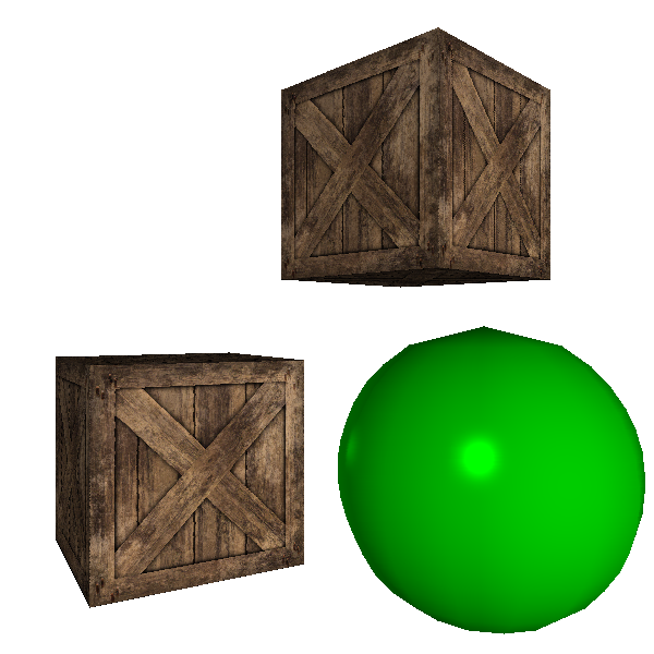
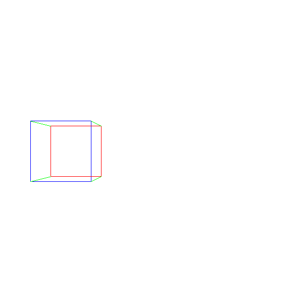
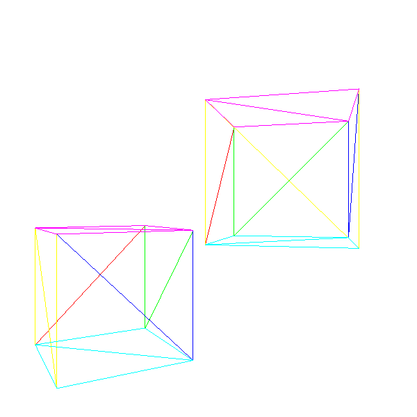
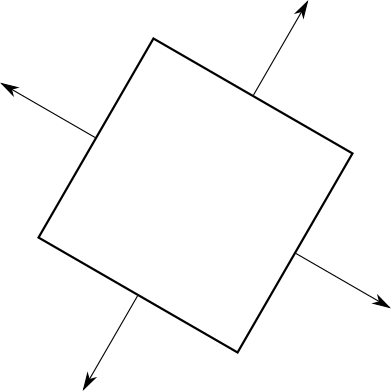
Therefore, we can move on and draw our first 3D object: a cube. We set the coordinates of its 8 vertices and draw the lines between the projections of 12 pairs of vertices that make up the edges of the cube:

  ViewportToCanvas(x, y) { return (x*Cw/Vw, y*Ch/Vh); } ProjectVertex(v) { return ViewportToCanvas(vx * d / vz, vy * d / vz) #  "" . vAf = [-1, 1, 1] vBf = [1, 1, 1] vCf = [1, -1, 1] vDf = [-1, -1, 1] #  "" . vAb = [-1, 1, 2] vBb = [1, 1, 2] vCb = [1, -1, 2] vDb = [-1, -1, 2] #  . DrawLine(ProjectVertex(vAf), ProjectVertex(vBf), BLUE); DrawLine(ProjectVertex(vBf), ProjectVertex(vCf), BLUE); DrawLine(ProjectVertex(vCf), ProjectVertex(vDf), BLUE); DrawLine(ProjectVertex(vDf), ProjectVertex(vAf), BLUE); #  . DrawLine(ProjectVertex(vAb), ProjectVertex(vBb), RED); DrawLine(ProjectVertex(vBb), ProjectVertex(vCb), RED); DrawLine(ProjectVertex(vCb), ProjectVertex(vDb), RED); DrawLine(ProjectVertex(vDb), ProjectVertex(vAb), RED); # ,     . DrawLine(ProjectVertex(vAf), ProjectVertex(vAb), GREEN); DrawLine(ProjectVertex(vBf), ProjectVertex(vBb), GREEN); DrawLine(ProjectVertex(vCf), ProjectVertex(vCb), GREEN); DrawLine(ProjectVertex(vDf), ProjectVertex(vDb), GREEN); 

And we get something like this:



Source code and working demo >>

Although it works, we have serious problems - what if we want to render two cubes? What if we want to render not something else, but something else? What if we do not know that we will render until the program is running - for example, load a 3D model from disk? In the next chapter, we will learn how to solve all these issues.

Scene settings

We developed techniques for drawing a triangle on the canvas according to given coordinates of its vertices and equations for converting the 3D coordinates of the triangle into 2D coordinates of the canvas. In this chapter, we learn how to represent objects consisting of triangles, and how to manipulate them.

For this we use a cube; This is not the easiest 3D object to create from triangles, but it will be useful to illustrate some of the problems. The edges of the cube have a length of two units and are parallel to the axes of coordinates, and its center is at the point of origin:



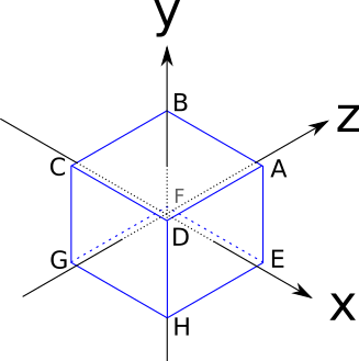
Here are the coordinates of its vertices:

$$$A = (1, 1, 1)$
$$$B = (-1, 1, 1)$
$$$C = (-1, -1, 1)$
$$$D = (1, -1, 1)$
$$$E = (1, 1, -1)$
$$$F = (-1, 1, -1)$
$$$G = (-1, -1, -1)$
$$H = ( 1 , - 1 , - 1 ) The sides of a cube are squares, but we only know how to handle triangles. There are no problems: any polygon can be decomposed into many triangles. Therefore, we represent each side of the cube in the form of two triangles.Of course, not any set of three vertices of a cube describes a triangle on the surface of the cube (for example, AGH is “inside” the cube), therefore the coordinates of its vertices are not enough to describe it; we also need to compile a list of triangles made up of these vertices:$H = (1, -1, -1)$

 A, B, C A, C, D E, A, D E, D, H F, E, H F, H, G B, F, G B, G, C E, F, B E, B, A C, G, H C, H, D 

This shows that there is a structure that can be used to represent any object made up of triangles: a list of coordinates of the vertices and a list of triangles that determines which set of three vertices forms the triangles of the object.

Each entry in the triangle list may contain additional information about the triangles; for example, we can store in it the color of each triangle.

Since two lists will be the most natural way to store this information, we use list indices as references to the list of vertices. That is, the above cube can be represented as follows:

 Vertexes 0 = ( 1, 1, 1) 1 = (-1, 1, 1) 2 = (-1, -1, 1) 3 = ( 1, -1, 1) 4 = ( 1, 1, -1) 5 = (-1, 1, -1) 6 = (-1, -1, -1) 7 = ( 1, -1, -1) Triangles 0 = 0, 1, 2, red 1 = 0, 2, 3, red 2 = 4, 0, 3, green 3 = 4, 3, 7, green 4 = 5, 4, 7, blue 5 = 5, 7, 6, blue 6 = 1, 5, 6, yellow 7 = 1, 6, 2, yellow 8 = 4, 5, 1, purple 9 = 4, 1, 0, purple 10 = 2, 6, 7, cyan 11 = 2, 7, 3, cyan 

To render an object presented in this way is quite simple: first, we project each vertex, save them in a temporary list of “projected vertices”; then we go through the list of triangles, rendering each individual triangle. In the first approximation, it will look like this:

 RenderObject(vertexes, triangles) { projected = [] for V in vertexes { projected.append(ProjectVertex(V)) } for T in triangles { RenderTriangle(T, projected) } } RenderTriangle(triangle, projected) { DrawWireframeTriangle(projected[triangle.v[0]], projected[triangle.v[1]], projected[triangle.v[2]], triangle.color) } 

We cannot simply apply this algorithm to the cube as it is, and hope for a correct mapping — some of the vertices are behind the camera; and this, as we have seen, leads to strange behavior. In fact, the camera is inside the cube.

So we just move the cube. To do this, we just need to move each vertex of the cube in one direction. Let's call this vector$$T , abbreviated from Translation. Let's just move the cube 7 units forward, so that it is exactly in front of the camera, and 1.5 units to the left, so that it looks more interesting. Since "forward" is the direction$T$$$→ Z + , and “left” -$\vec{Z_+}$$$→ X - , then the displacement vector will have the following form$\vec{X-}$

$$

$$\vec{T} = \begin{pmatrix} -1.5 \\ 0 \\ 7 \end{pmatrix}$$

To get the moved version $$V ′ of each point$V'$$$V cube, we just need to add the displacement vector:$V$

$$

$$V' = V + \vec{T}$$

At this stage, we can take a cube, move each vertex, and then apply the above algorithm to finally get our first 3D cube:



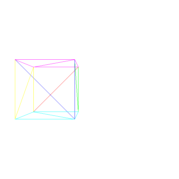
Source code and working demo >>

Models and instances

But what if we need to render two cubes?

A naive approach would be to create another set of vertices and triangles describing the second cube. It will work, but it will take a lot of memory. And if we want to render a million cubes?

It will be smarter to think in categories of models and instances . A model is a set of vertices and triangles that describes an object as it is (that is, "a cube consists of the following set of vertices and triangles "). On the other hand, an instance of a model is a concrete implementation of the model at some position of the scene (that is, “ there is a cube in (0, 0, 5) ”).

The advantage of the second approach is that each object in the scene is sufficient to specify only once, after which an arbitrary number of instances can be placed in the scene simply by describing their positions within the scene.

Here is a rough approximation of how such a scene can be described:

 model { name = cube vertexes { ... } triangles { ... } } instance { model = cube position = (0, 0, 5) } instance { model = cube position = (1, 2, 3) } 

To render it, we just need to go through the list of instances; for each instance, create a copy of the model vertices, apply the instance position to them, and then act as before:

 RenderScene() { for I in scene.instances { RenderInstance(I); } } RenderInstance(instance) { projected = [] model = instance.model for V in model.vertexes { V' = V + instance.position projected.append(ProjectVertex(V')) } for T in model.triangles { RenderTriangle(T, projected) } } 

Note that in order for this algorithm to work, the coordinates of the model vertices must be defined in a coordinate system “logical” for the object (this is called the model space ). For example, a cube is defined in such a way that its center is at (0, 0, 0); this means that when we say "the cube is located at (1, 2, 3) ", we mean "the cube is centered relative to (1, 2, 3) ". There are no hard and fast rules for defining model space; mainly depends on the application. For example, if you have a human model, then it is logical to locate the origin point at the soles of his feet. The moved vertices will now be expressed in the "absolute" coordinate system of the scene (called the space of the world ).

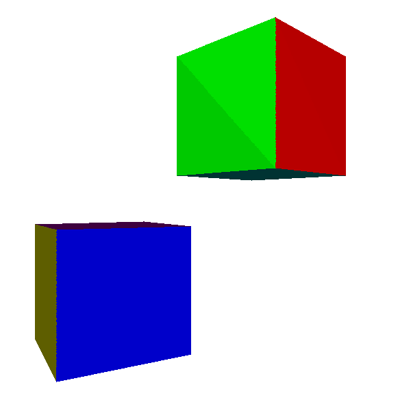
Here are two cubes:



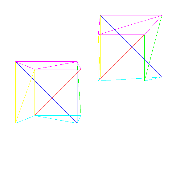
Source code and working demo >>

Model conversion

The above scene definition limits us quite a lot; in particular, since we can only specify the position of the cube, we are able to create as many instances as possible of the cubes, but they will all be oriented in the same way. In general, we need to have more control over the instances; we also want to set their orientation, and possibly their scale.

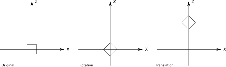
Conceptually, we can define the transformation of the model with exactly these three elements: the scale factor, the rotation relative to the point of origin of the model space and the movement to a certain point of the scene:

 instance { model = cube transform { scale = 1.5 rotation = <45 degrees around the Y axis> translation = (1, 2, 3) } } 

You can easily extend the previous version of the pseudocode by adding new transformations. However, the order of application of these transformations is important; in particular, the movement must be performed last. Here's a twist on$$45 ∘ around the origin point, followed by the movement along the Z axis:But the movement applied before the turn:We can write a more general version:$45^\circ$







RenderInstance()

 RenderInstance(instance) { projected = [] model = instance.model for V in model.vertexes { V' = ApplyTransform(V, instance.transform); projected.append(ProjectVertex(V')) } for T in model.triangles { RenderTriangle(T, projected) } } 

The method is ApplyTransform()as follows:

 ApplyTransform(vertex, transform) { V1 = vertex * transform.scale V2 = V1 * transform.rotation V3 = V2 + transform.translation return V3 } 

Rotation is expressed as a 3x3 matrix; if you are not familiar with the rotation matrices, for now consider that any 3D rotation can be represented as a product of a point and a 3x3 matrix. See more about linear algebra.

Camera conversion

In the previous sections, we learned how to place instances of models at different points in the scene. In this section, we will learn how to move and rotate the camera in the scene.

Imagine that you are hanging in the middle of a completely empty coordinate system. Everything is painted black. Suddenly a red cube appears right in front of you. A moment later, the cube comes one unit closer to you. But did the cube come close to you? Or did you yourself move one unit to the cube?

Since we have no starting point, and the coordinate system is not visible, we can not determine what happened.

Now the cube has turned around you on$$45 ∘ clockwise.$45^\circ$ But is it? Perhaps it was you turned around on him $$45 ∘ counterclockwise? We again can not determine this.This thought experiment shows us that there is no difference between moving the camera in a fixed scene and a fixed camera in the moving and turning around the scene!The advantage of this obviously selfish vision of the universe is that with a camera fixed at the origin point, the camera is looking in the direction$45^\circ$



$$→ Z + , we can immediately use the projection equations derived in the previous chapter without any changes. The coordinate system of the camera is calledthe camera space. We assume that the camera also has a transformation consisting of moving and turning (we will lower the scale). In order to render the scene from the point of view of the camera, we need to apply inverse transformations to each vertex in the scene:$\vec{Z_+}$

 V1 = V - camera.translation V2 = V1 * inverse(camera.rotation) V3 = perspective_projection(V2) 

Transformation matrix

Let's take a step back and see what happens to the top. $$V in the model space until it is projected to a point on the canvas$V$$$$(cx, cy)$ .

First we apply the model transformation to go from the model space to the space of the world:

 V1 = V * instance.rotation V2 = V1 * instance.scale V3 = V2 + instance.translation 

Then we apply the camera transform to go from the space of the world to the space of the camera:

 V4 = V3 - camera.translation V5 = V4 * inverse(camera.rotation) 

Then we apply the perspective equations:

 vx = V5.x * d / V5.z vy = V5.y * d / V5.z 

Finally, we bind the coordinates of the viewport to the coordinates of the canvas:

 cx = vx * cw / vw cy = vy * ch / vh 

As you can see, this is a fairly large amount of computation and for each vertex a set of intermediate values ​​is calculated. Wouldn't it be convenient if we cut it all down to a single matrix product — take$$V , multiply it by some matrix and get directly$V$$$$cx$ with $$$cy$ ?

Let's express the transformations in the form of functions that receive a vertex and return a transformed vertex. Let be $$$C_T$ and $$C R will be moving and turning the camera,$C_R$$$$I_R$ , $$$I_S$ and $$I T - rotation, scale and movement of the instance,$I_T$$$P - perspective projection, and$P$$$M - by placing the preview window on the canvas.$M$ If a $$V is the initial vertex, and$V$$$V ′ is a point on the canvas, then we can express all the above equations as follows:$V'$

$$

$$V' = M(P(C_R^{-1}(C_T^{-1}(I_T(I_S(I_R(V)))))))$$

Ideally, we would like to have a single transformation that performs the same as a series of source transformations, but has a much simpler expression:

$$

$$F = M \cdot P \cdot C_R^{-1} \cdot C_T^{-1} \cdot I_T \cdot I_S \cdot I_R$$

$$

$$V' = F(V)$$

Finding a single matrix representing $$F is a nontrivial task. The main problem is that transformations are expressed in various ways: displacement is the sum of a point and a vector, rotation and scale are the product of a point and a 3x3 matrix, and in the perspective projection division is used. But if we can express all the transformations in one way, and this way will have a simple mechanism for creating transformations, then we will get what we need.$F$

Homogeneous coordinates

Consider the expression $$$A = (1, 2, 3)$ . $$A is a 3D-point or a 3D-vector? There is no way of knowing this without additional context. But let's accept the following arrangement: we will add to the presentation a fourth component, called$A$

$$$w$ . If a $$w = 0 , then we are talking about a vector.$w = 0$ If a $$w = 1 , then we are talking about a point. That is the point$w = 1$$$A is unambiguously represented as$A$$$A = ( 1 , 2 , 3 , 1 ) , and vector$A = (1, 2, 3, 1)$$$→ A is represented as$\vec{A}$$$$(1, 2, 3, 0)$ .Since points and vectors have a general idea, this is called homogeneous coordinates (Note: homogeneous coordinates have a much deeper and more detailed geometric interpretation, but it does not belong to the subject of our article; here we simply use them as a convenient tool with certain properties.).

Such a representation has a large geometric meaning. For example, by subtracting two points, you get a vector:

$$

$$(8, 4, 2, 1) - (3, 2, 1, 1) = (5, 2, 1, 0)$$

Adding two vectors yields a vector:

$$

$$(0, 0, 1, 0) + (1, 0, 0, 0) = (1, 0, 1, 0)$$

Similarly, you can easily see that by summing a point and a vector, we get a point, multiplying a vector by a scalar gives a vector, and so on.

And what are the coordinates with$$w not equal to either$w$$$0 , no$0$$$$1$ ?They also represent points; in fact, any point in 3D has an infinite number of representations in homogeneous coordinates. The relationship between the coordinates and the value is important.$$$w$ ; i.e, $$$(1, 2, 3, 1)$ and $$( 2 , 4 , 6 , 2 ) represent the same point as$(2, 4, 6, 2)$$$$(-3, -6, -9, -3)$ .

Of all these representations, we can call the presentation with $$w = 1 by the canonical representation of apoint in homogeneous coordinates; Converting any other representation to its canonical representation or to Cartesian coordinates is a trivial task:$w = 1$

$$

$$\begin{pmatrix} x \\ y \\ z \\ w \end{pmatrix} = \begin{pmatrix}{c} x \over w \\ y \over w \\ z \over w \\ 1 \end{pmatrix} = \begin{pmatrix} x \over w \\ y \over w \\ z \over w \end{pmatrix}$$

That is, we can convert Cartesian coordinates to homogeneous coordinates, and back to Cartesian coordinates. But how does this help us find a single view for all transformations?

Uniform rotation matrix

Let's start with the rotation matrix. The expression of the Cartesian 3x3 rotation matrix in homogeneous coordinates is trivial; since the coordinate$$w points should not change, we will add a column to the right, a row at the bottom, fill them with zeros and place them in the bottom right element$w$$$1 to store value$1$$$$w$ :

$$

$$\begin{pmatrix} A & B & C \\ D & E & F \\ G & H & I \end{pmatrix} . \begin{pmatrix} x \\ y \\ z \end{pmatrix} = \begin{pmatrix} x' \\ y' \\ z' \end{pmatrix} \rightarrow \begin{pmatrix} A & B & C & 0 \\ D & E & F & 0 \\ G & H & I & 0 \\ 0 & 0 & 0 & 1 \end{pmatrix} . \begin{pmatrix} x \\ y \\ z \\ 1 \end{pmatrix} = \begin{pmatrix} x' \\ y' \\ z' \\ 1 \end{pmatrix}$$

The scaling matrix is ​​also trivial in homogeneous coordinates, and it is created in the same way as the rotation matrix:

$$

$$\begin{pmatrix} S_x & 0 & 0 \\ 0 & S_y & 0 \\ 0 & 0 & S_z \end{pmatrix} . \begin{pmatrix} x \\ y \\ z \end{pmatrix} = \begin{pmatrix} x \cdot S_x \\ y \cdot S_y \\ z \cdot S_z \end{pmatrix} \rightarrow \begin{pmatrix} S_x & 0 & 0 & 0 \\ 0 & S_y & 0 & 0 \\ 0 & 0 & S_z & 0 \\ 0 & 0 & 0 & 1 \end{pmatrix} . \begin{pmatrix} x \\ y \\ z \\ 1 \end{pmatrix} = \begin{pmatrix} x \cdot S_x \\ y \cdot S_y \\ z \cdot S_z \\ 1 \end{pmatrix}$$

Uniform translation matrix

The previous examples were simple; they were already presented as matrix multiplications in Cartesian coordinates, it was enough for us to add$$1 to save the coordinate$1$$$$w$ .But what do we do with the displacement, which we expressed in Cartesian coordinates as addition?

We need a 4x4 matrix such that

$$

$$\begin{pmatrix} T_x \\ T_y \\ T_z \\ 0 \end{pmatrix} + \begin{pmatrix} x \\ y \\ z \\ 1 \end{pmatrix} = \begin{pmatrix} A & B & C & D \\ E & F & G & H \\ I & J & K & L \\ M & N & O & P \end{pmatrix} . \begin{pmatrix} x \\ y \\ z \\ 1 \end{pmatrix} = \begin{pmatrix} x + T_x \\ y + T_y \\ z + T_z \\ 1 \end{pmatrix}$$

Let's first focus on getting $$$x + T_x$ . This value is the result of multiplying the first row of the matrix by a point, that is,

$$

$$\begin{pmatrix} A & B & C & D \end{pmatrix} . \begin{pmatrix} x \\ y \\ z \\ 1 \end{pmatrix} = x + T_x$$

If we open the vector product, we get

$$

$$Ax + By + Cz + D = x + T_x$$

And from this we can infer that $$$A = 1$ , $$$B = C = 0$ , but $$$D = T_x$ .

Applying the same reasoning to the remaining coordinates, we obtain the following matrix expression for the displacement:

$$

$$\begin{pmatrix} T_x \\ T_y \\ T_z \\ 0 \end{pmatrix} + \begin{pmatrix} x \\ y \\ z \\ 1 \end{pmatrix} = \begin{pmatrix} 1 & 0 & 0 & T_x \\ 0 & 1 & 0 & T_y \\ 0 & 0 & 1 & T_z \\ 0 & 0 & 0 & 1 \end{pmatrix} . \begin{pmatrix} x \\ y \\ z \\ 1 \end{pmatrix} = \begin{pmatrix} x + T_x \\ y + T_y \\ z + T_z \\ 1 \end{pmatrix}$$

The sum and product can be simply expressed as the products of matrices and vectors, which are sums and products. But in the perspective projection equations, division by$$$z$ .How to express it?

There is a great temptation to find that the division into$$z is the same as multiplying by$z$$$1 / z , which is actually true; but in our case it is useless because the coordinate$1/z$$$The specificpoint z cannot be located in the projection matrix applied toeachpoint. Fortunately, in homogeneous coordinates there is one case of division: division by coordinate$z$

$$w when converting to Cartesian coordinates. So there we will manage to turn the coordinate$w$$$z reference point in coordinate$z$$$w "projected" point, then we get the projected$w$$$$x$ and $$y after converting the point back to Cartesian coordinates:$y$

$$

$$\begin{pmatrix} A & B & C & D \\ E & F & G & H \\ I & J & K & L \end{pmatrix} . \begin{pmatrix} x \\ y \\ z \\ 1 \end{pmatrix} = \begin{pmatrix} x.d \\ y.d \\ z \end{pmatrix} \rightarrow \begin{pmatrix} x.d \over z \\ y.d \over z \end{pmatrix}$$

Note that this matrix has the size $$$3\times 4$ ; it can be multiplied by a four-element vector (transformed 3D point in homogeneous coordinates), thus obtaining a three-element vector (projected 2D point in homogeneous coordinates), which is then converted into two-dimensional Cartesian coordinates by dividing by $$$w$ . This will give us exact values. $$$x '$ and $$y ′ that we are looking for. Not enough here$y '$

$$z ′ , which, as we know, is by definition$z'$$$$d$ .

Using reasoning similar to those we used to derive the translation matrix, we can express the perspective projection as

$$

$$\begin{pmatrix} d & 0 & 0 & 0 \\ 0 & d & 0 & 0 \\ 0 & 0 & 1 & 0 \end{pmatrix} . \begin{pmatrix} x \\ y \\ z \\ 1 \end{pmatrix} = \begin{pmatrix} x.d \\ y.d \\ z \end{pmatrix} \rightarrow \begin{pmatrix} x.d \over z \\ y.d \over z \end{pmatrix}$$

Uniform matrix from a window of viewing on a canvas

The last stage is the placement of the point projected onto the viewing window on the canvas. This is just a two-dimensional scale conversion with$$$S_x = c_w \over v_w$ and $$$S_y = c_h \over v_h$ . That is, the matrix will be next

$$

$$\begin{pmatrix} c_w \over v_w & 0 & 0 \\ 0 & c_w \over v_w & 0 \\ 0 & 0 & 1 \end{pmatrix} . \begin{pmatrix} x \\ y \\ z \end{pmatrix} = \begin{pmatrix} x.c_w \over v_w \\ y.c_h \over v_h \\ z \end{pmatrix}$$

In fact, it is easy to combine it with a projection matrix and get a simple transformation matrix from 3D to canvas:

$$

$$\begin{pmatrix} d.cw \over vw & 0 & 0 & 0 \\ 0 & d.ch \over vh & 0 & 0 \\ 0 & 0 & 1 & 0 \end{pmatrix} . \begin{pmatrix} x \\ y \\ z \\ 1 \end{pmatrix} = \begin{pmatrix} x.d.cw \over vw \\ y.d.cw \over vh \\ z \end{pmatrix} \rightarrow \begin{pmatrix} ({x.d \over z})({cw \over vw}) \\ ({y.d \over z})({ch \over vh}) \end{pmatrix}$$

Practical use

For practical reasons, we will not use the projection matrix. Instead, we use model and camera transformations, and then convert their results back to Cartesian coordinates as follows:

$$

$$x' = {x.d.cw \over z.vw}$$

$$

$$y' = {y.d.ch \over z.vh}$$

This will allow us to perform other operations in 3D before projecting points, which cannot be expressed as matrix transformations.

Again the transformation matrix

Since we can now express any 3D transformation of the original vertex $$V , performed before projecting as a 4x4 matrix, we can trivially combine all these transformations into a single 4x4 matrix by multiplying them:$V$

$$

$$F = C_R^{-1}.C_T^{-1}.I_T.I_S.I_R$$

And then the vertex transformation is simply a matter of calculating the following work:

$$

$$V' = F.V$$

Moreover, we can decompose the transformation into two parts:

$$

$$M_{Camera} = C_R^{-1}.C_T^{-1}$$

$$

$$M_{Model} = I_T.I_S.I_R$$

$$

$$M = M_{Camera}.M_{Model}$$

These matrices do not need to be calculated for each vertex (this is the meaning of using the matrix). In fact, they do not even have to be calculated in each frame.

$$M C a m e r a may change every frame; it depends on the camera position and orientation, so if the camera moves or rotates, then it must be recalculated. However, after the calculation, it remains constant for each object drawn in the frame, so it will be calculated at most once per frame.$M_{Camera}$

$$M M o d e l depends upon conversion model instance and therefore used the matrix will change only once for an object in the scene; however, it will remain constant for fixed objects (for example, trees, buildings), so it can be calculated in advance and stored in the scene itself. For moving objects (for example, for cars in a racing game), it must still be calculated every time they move (usually in each frame).At a very high level, the pseudo-code for rendering the scene will look like this:$M_{Model}$

 RenderModel(model, transform) { projected = [] for V in model.vertexes { projected.append(ProjectVertex(transform * V)) } for T in model.triangles { RenderTriangle(T, projected) } } RenderScene() { MCamera = MakeCameraMatrix(camera.position, camera.orientation) for I in scene.instances { M = MCamera*I.transform RenderModel(I.model, M) } } 

Now we can draw a scene containing several instances of various models, possibly moving and turning, and we can move the camera around the scene.



Source code and working demo >>

We have made a big step forward, but we still have two important limitations. First, when the camera moves, objects may end up behind it, which creates all sorts of problems. Secondly, the result of rendering does not look very good: it is still framed.

In the next chapter, we will deal with objects that should not be visible, and then spend the remaining time improving the appearance of rendered objects.

Clipping

In the chapter Perspective projection, we obtained the following equations:

$$

$$P'_X = {P_X \cdot d \over P_Z}$$

$$

$$P'_Y = {P_Y \cdot d \over P_Z}$$

Division by $$P Z causes problems; when it can divide by zero. It can also result in negative values ​​representing points behind the camera that are processed incorrectly. Even the points in front of the camera, but very close, can cause problems in the form of highly distorted objects. To avoid all these problem cases, we decided not to render anything beyond the projection plane.$P_Z$

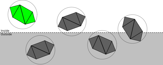
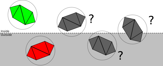
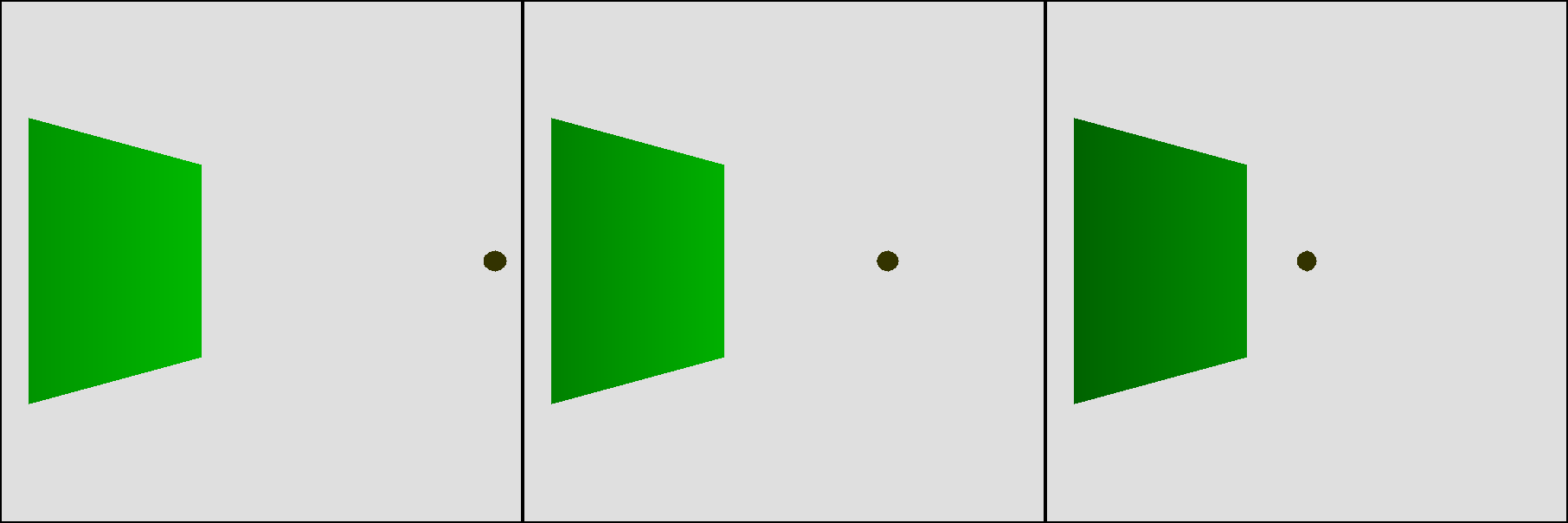
$$$Z = d$ .This clipping plane allows you to divide all the points into the clipping inside or outside the volume , that is, the subsets of the space that is actually visible from the camera. In this case, the cutoff volume is the " half space in front $$Z = d ". We render only parts of the scene that are inside the clipping volume.The fewer operations we do, the faster our renderer will be, so we use the top-down approach. Consider a scene with several objects, each of which consists of four triangles.At each stage, we strive to determine, as little as possible, whether clipping can be stopped at this point, or further and more detailed clipping is required:$Z = d$

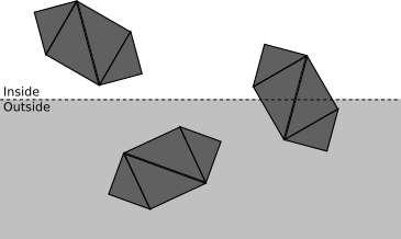
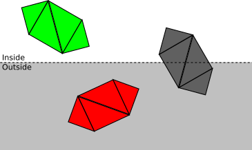
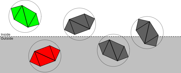
• If the object is completely inside the clipping volume, then it is accepted (highlighted in green); if it is completely outside, it is discarded (red):

• Otherwise, we repeat the process for each triangle. If the triangle is completely inside the volume of the cut-off, then it is accepted; if completely outside, it is discarded:

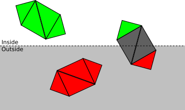
• Otherwise, we need to break the triangle itself. The original triangle is discarded, and one or two triangles are added, covering the part of the triangle inside the cut-off volume:

Now we will take a closer look at each stage in the process.

Defining clipping planes

The first thing to do is to find the equation of the clipping plane. There is nothing wrong with$$Z = d , but this is not the most convenient format for our purposes; later in this chapter, we will develop a more general approach to other clipping planes, so we need to come up with a general approach instead of this particular case. The general equation of a 3D plane is$Z = d$

$$$Ax + By + Cz + D = 0$ . It means that the point $$P = ( x , y , z ) will satisfy the equation if and only if$P = (x, y, z)$$$P is on the plane. We can rewrite the equation as$P$$$$\langle \vec{N}, P \rangle + D = 0$ where $$$\vec{N} = (A, B, C)$ .

Notice that if $$$\langle \vec{N}, P \rangle + D = 0$ then $$k ⟨ → N , P ⟩ + k D = 0 for any value of$k\langle \vec{N}, P \rangle + kD = 0$$$$k$ . In particular, we can choose $$k = 1| → N | and get a new equation$k = { 1 \over |\vec{N}| }$$$$\langle \vec{N}', P \rangle + D' = 0$ where $$→ N ′is the unit vector. That is, for any given plane, we can assume that there is a unit vector$\vec{N}'$$$→ N and real number$\vec{N}$$$$D$ such that $$⟨ → N , P ⟩ + D = 0  is the equation of this plane. This is a very convenient wording:$\langle \vec{N}, P \rangle + D = 0\$

$$→ N is actually the normal of the plane, and$\vec{N}$$$- D - distance with a sign from the point of origin of coordinates to the plane. In fact, for any point$-D$$$$P$$$⟨ → N , P ⟩ + D is the distance from the sign of$\langle \vec{N}, P \rangle + D$$$P to the plane; easy to see that$P$$$0 is a special case in which$0$$$P lies on the plane. As we saw earlier, if$P$

$$→ N is the normal to the plane, like$\vec{N}$$$→ - N , so we choose$\vec{-N}$$$→ N such that it is directed “inside” the cut-off volume. For the plane$\vec{N}$$$Z = d we choose the normal$Z = d$$$( 0 , 0 , 1 ) , which is directed "forward" relative to the camera. Since the point$(0, 0, 1)$$$( 0 , 0 , d ) lies on the plane, it must satisfy the equation of the plane, we can calculate it, knowing$(0, 0, d)$$$$D$ :

$$

$$\langle \vec{N}, P \rangle + D = \langle (0, 0, 1), (0, 0, d) \rangle + D = d + D = 0$$

i.e $$D = - d (Note: you could trivially get this from$D = -d$$$Z = d , rewriting it as$Z = d$$$$Z - d = 0$ . However, the reasoning presented here applies to all other planes with which we will deal, and this allows us to cope with the fact that $$- Z + d = 0 is also valid, but the normal is directed in the wrong direction.).$-Z + d = 0$

Cut-off volume

Although using a single clipping plane to ensure that the objects behind the camera are not rendered, we get the right results, this is not entirely effective. Some objects may be in front of the camera, but still not be visible; for example, the projection of an object near the projection plane, but located very far to the right, will fall out of the viewing window, and therefore will be invisible:



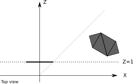
All the resources that we use to calculate the projection of such an object, as well as calculations for triangles and vertices, performed for its rendering, will be wasted. It will be much more convenient for us to completely ignore such objects.

Fortunately, it is not difficult at all. We can define additional planes that cut the scene smoothly.to the point that will be visible from the viewing window; such planes are defined by the camera and both sides of the viewing window:



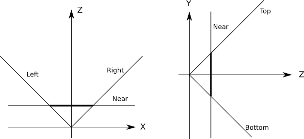
All these planes have$$D = 0 (because the origin point is on all planes), so we can only determine the normals. The simplest case is FOV.$D = 0$$$90 ∘ , at which the planes are at$90^\circ$$$45 ∘ , so their normals$45^\circ$$$( 1√2 ,0,1√2 )for the left plane,$({1 \over \sqrt{2}}, 0, {1 \over \sqrt{2}})$$$( - 1√2 ,0,1√2 )for the right plane,$({-1 \over \sqrt{2}}, 0, {1 \over \sqrt{2}})$$$( 0 , 1√2 ,1√2 )for the bottom and$(0, {1 \over \sqrt{2}}, {1 \over \sqrt{2}})$$$( 0 , - 1√2 ,1√2 )for the upper planes. To calculate clipping planes for any arbitrary FOV, only a small amount of trigonometric calculations are required. To cut off objects or triangles in terms of the cut-off volume, we just need to cut them in order by each plane. All objects “surviving” after being cut off by one plane are cut off by the other planes; this works because the clipping volume is the intersection of the half-spaces defined by each clipping plane.$(0, {-1 \over \sqrt{2}}, {1 \over \sqrt{2}})$

Clipping whole objects

Fully specifying the volume of the clipping with its clipping planes, we can begin by determining whether the object is completely inside or outside the half-space defined by each of these planes.

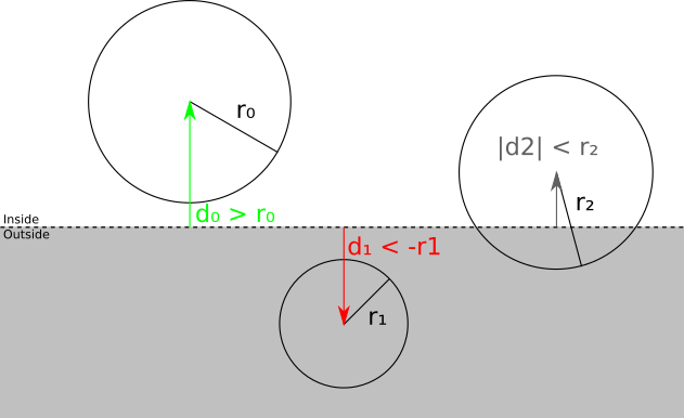
Suppose we put each model inside the smallest sphere that can contain it. We will not discuss in the article how this can be done; the sphere can be calculated from a set of vertices by one of several algorithms, or the approximation can be given by the model developer. In any case, we will assume that we have a center$$C and radius$C$$$r spheres that completely contains each object:We can split the spatial relationship between the sphere and the plane into the following categories:$r$

• . ; ( ):

• . ; ( , — ):

• . , ; , , . .

How is this categorization actually performed? We have chosen a way of expressing cut-off planes in such a way that the substitution of any point in the equation of a plane gives us a distance with a sign from a point to a plane; in particular, we can calculate the distance with the sign$$d from the center of the bounding sphere to the plane. Therefore, if$d$$$d > r , then the sphere is in front of the plane;$d > r$ if a $$d < - r , then the sphere is behind the plane; otherwise$d < -r$$$d | < r , that is, the plane intersects the sphere.$d| < r$

Triangle Triangle

If the verification of the sphere-plane is not enough to determine whether the object is completely in front of or completely behind the clipping plane, then each triangle should be cut off relative to it.

We can classify each vertex of the triangle relative to the clipping plane by taking the sign of the distance with a sign to the plane. If the distance is zero or positive, then the vertex is in front of the clipping plane, otherwise - behind it:



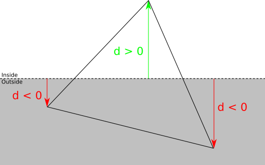
There are four possible cases:

• Three peaks are in front of the plane. In this case, the entire triangle is in front of the clipping plane, so it is accepted without further clipping with respect to this plane.
• . , .
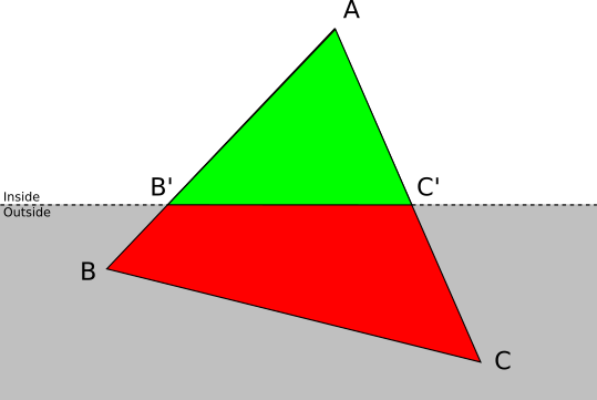
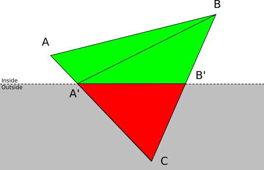
• . Let be $$$A$ — $$$ABC$ , . In this case $$$ABC$ , $$$AB'C'$ where $$$B'$ and $$$C'$ — $$$AB$ and $$$AC$ .

• . Let be $$$A$ and $$$B$ — $$$ABC$ , . ABC , : $$$ABA'$ and $$$A'BB'$ where $$$A'$ and $$$B'$ — $$$AC$ and $$$BC$ .

To perform clipping for each triangle, we need to calculate the intersection of the sides of the triangle with the clipping plane. It should be noted that it is not enough to calculate the coordinates of the intersection: it is also necessary to calculate the corresponding value of the attributes associated with the vertices, for example, shading, which we did in the chapter Drawing Shaded Triangles , or one of the attributes described in subsequent chapters.

We have a clipping plane given by the equation$$$\langle N, P \rangle + D = 0$ . Side of the triangle $$A B can be expressed using a parametric equation as$AB$$$$P = A + t(B - A)$ at $$$0 \le t \le 1$ . To calculate the value of a parameter $$t at which the intersection occurs, we will replace$t$$$P in the equation of the plane on the parametric equation of the segment:$P$

$$

$$\langle N, A + t(B - A) \rangle + D = 0$$

Using the linear properties of the scalar product, we obtain:

$$

$$\langle N, A \rangle + t\langle N, B - A \rangle + D = 0$$

Calculate $$$t$ :

$$

$$t = {-D - \langle N, A \rangle \over \langle N, B - A \rangle}$$

We know that a solution always exists, because $$A B intersects the plane; mathematically$AB$$$⟨ N , B - A ⟩ can not be zero, because this would mean that the segment and the normal perpendicular to that in turn implies that the segment and the plane do not intersect. Calculating$\langle N, B - A \rangle$

$$t , we get that intersection$t$$$Q is just equal$Q$

$$

$$Q = A + t(B - A)$$

Notice that $$t is part of the segment$t$$$A B where the intersection occurred.$AB$ Let be $$$\alpha_A$ and $$α B will be the values ​​of some attribute$\alpha_B$$$ a l p h a in points$\ alpha$$$$A$ and $$$B$ ; if we assume that the attribute varies linearly along $$$AB$ then $$α Q can be simply calculated as$\alpha_Q$

$$

$$\alpha_Q = \alpha_A + t(\alpha_B - \alpha_A)$$

Clipping in pipeline

The order of the chapters of the article does not correspond to the order of operations performed in the rendering pipeline; As explained in the introduction, the chapters are arranged in such a way that visual progress can be made as quickly as possible.

Clipping is a 3D operation; it receives two 3D objects in the scene and generates a new set of 3D objects in the scene, namely, the intersection of the scene and the clipping volume. It should be clear that clipping should be performed after objects have been placed in the scene (that is, vertices are used after the model and camera transformations), but before a perspective projection.

The techniques presented in this chapter work reliably, but they are very common. The more we know in advance about the scene, the more effective the clipping will be. For example, many games pre-process game maps, adding visibility information to them; if you manage to divide the scene into “rooms”, you can create a table listing the rooms visible from each specific room. When rendering the scene in the future, you just need to find out which room the camera is in, after which you can ignore all the rooms marked as “invisible” from it, saving considerable resources during rendering. Of course, at the same time you have to spend more time on pre-processing, and the scene turns out to be more rigidly defined.

Removing hidden surfaces

Now that we can render any scene from any vantage point, let's enhance our wireframe graphics.

The obvious first step is to give solid objects a solid appearance. To do this, let's use a DrawFilledTriangle()random color to draw each triangle, and see what happens: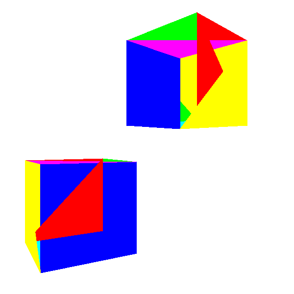



Not very much like cubes, right?

The problem here is that some triangles that should be behind others are drawn in front of them. Why?Because we simply draw 2D triangles on the canvas in almost random order - in the order that we got when defining the model.

However, when specifying the triangles of the model, there is no “correct” order. Suppose that the triangles of the model are sorted in such a way that the back faces are drawn first, and then they are overlapped by the front faces. We will get the expected result. However, if we turn the cube on$$180 ∘ , we get the opposite situation - long triangles will overlap near.$180^\circ$

Algorithm of the artist

The first solution to this problem is known as the " artist algorithm ". Artists in the real world first draw the background and then cover its parts with the front objects. We can achieve the same effect by taking each scene triangle, applying model and camera transformations, sorting them back to front and drawing them in that order.

While the triangles are drawn in the correct order, this algorithm has drawbacks that make it impractical.

Firstly, it does not scale well. The best sorting algorithm has speed$$O ( n . L o g ( n ) ) \), i.e. the execution time of more than doubled by doubling the number of triangles. In other words, it works for small scenes, but quickly becomes a bottleneck as the complexity of the scene increases.Secondly, it requires the simultaneous knowledge of the entire list of triangles. This requires a lot of memory, and does not allow the use of streaming approach to rendering. If you consider rendering as a conveyor, in which model triangles enter from one end, and pixels go from the other, it is impossible to start outputting pixels until each triangle is processed. In turn, this means that we cannot parallelize this algorithm.$O(n.log(n))$



Thirdly, even if you put up with these restrictions, there are still cases where the correct order of the triangles does not exist. Consider the following case:



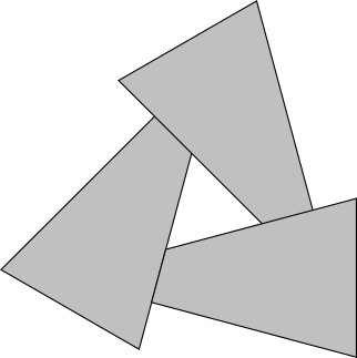
No matter in what order you will draw these triangles - you will always get the wrong result.

Depth buffer

If the solution of the problem at the level of triangles does not work, then the solution at the level of pixels will work exactly, and at the same time it overcomes all the limitations of the artist's algorithm.

In essence, we want to paint each pixel of the canvas with the “right” color. In this case, the “correct” color is the color of the object closest to the camera (in our case$$$P_1$ ):



It turns out that we can easily do this. Suppose we store the value$$The z points currently represented by each pixel of the canvas. When we decide whether to fill a pixel with a certain color, we do this only when the coordinate$Z$$$Z points we are going to paint over, less coordinates$Z$$$Z point, which is already there. Imagine an order of triangles in which we first want to paint$Z$

$$P 2 and then$P_2$$$$P_1$ . The pixel is painted red, its $$Z is marked as$Z$$$$Z_{P_2}$ . Then we paint over $$P 1 and since$P_1$$$Z P 2 > Z P 1 , the pixel is overwritten in blue; we get the right results. Of course, we got the right result, regardless of the values$Z_{P_2} > Z_{P_1}$

$$$Z$ . What if we wanted to paint first $$P 1 and then$P_1$$$$P_2$ ? Pixel first painted in blue, and $$Z P 1 preserved; but then we want to paint over$Z_{P_1}$$$P 2 and since$P_2$$$Z P 2 > Z P 1 , we will not paint it (because if we did, we would paint over the remote point, closing the closer one). We get a blue pixel again, which is the correct result. In terms of implementation, we need a buffer to store the coordinates.$Z_{P_2} > Z_{P_1}$

$$Z of each pixel on the canvas; it is calleda depth buffer, and its dimensions are naturally equal to the size of the canvas. But where do the values ​​come from?$Z$

$$$Z$ ?

They must be values $$Z points after conversion, but before perspective projection. That is why, in the chapterConfiguring the Scene,we defined the transformation matrices so that the final result contains$Z$$$$1/Z$ .

So we can get the values $$Z of these values$Z$$$$1/Z$ .But we only have this value for vertices; we need to get it for every pixel.

And this is another way to use the attribute assignment algorithm. Why not use$$Z as an attribute and not interpolate it along the edge of a triangle? You already know the procedure; we take values,and, we calculate,and, we receive from themand, and then we calculatefor each pixel of each horizontal segment. And instead of doing blindly,we do the following:$Z$Z0Z1Z2Z01Z02Z02z_leftz_rightz_segmentPutPixel(x, y, color)

 z = z_segment[x - xl] if (z < depth_buffer[x][y]) { canvas.PutPixel(x, y, color) depth_buffer[x][y] = z } 

For this to work, it depth_buffermust be initialized with values.$$+ ∞ (or simply “very large value”). The results obtained are now much better:Source code and working demo >>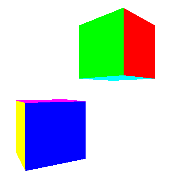$+\infty$

Why 1 / Z instead of Z

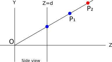
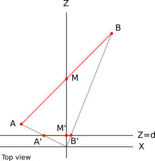
But the story does not end there. Meanings $$Z vertices are correct (after all, they are obtained from data), but in most cases linearly interpolated values$Z$$$Z for the remaining pixels will be incorrect. Although this approximation is “good enough” for buffering depths, in the future it will interfere. To check how wrong the values ​​are, consider the simple case of a straight line from$Z$

$$$A (-1, 0, 2)$ at $$$B (1, 0, 10)$ . Mid section $$M has coordinates$M$$$$(0, 0, 6)$ :



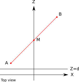
Let's calculate the projection of these points by $$$d = 1$ . $$$A'_x = A_x / A_z = -1 / 2 = -0.5$ . Similarly $$$B'_x = 0.1$ and $$$M'_x = 0$ :



What happens now if we linearly interpolate the values $$$A_z$ and $$B z to get the calculated value for$B_z$$$$M_z$ ?The linear function looks like this:



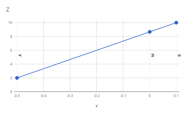
From this we can conclude that

$$

$${ M_z - A_z \over M'_x - A'_x } = { B_z - A_z \over B'_x - A'_x }$$

$$

$$M_z = A_z + (M'_x - A'_x) ({B_z - A_z \over B'_x - A'_x})$$

If we substitute numbers and perform arithmetic calculations, we get

$$

$$M_z = 2 + (0 - (-0.5))({10 - 2 \over 0.1 - (-0.5)}) = 2 + (0.5)({8 \over 0.6}) = 8.666$$

which is obviously not equal$$$M_z = 6$ .

So what's the problem? We use attribute assignment, which we know works well; we give it the correct values ​​that are obtained from the data; so why are the results wrong?

The problem is that we implicitly mean performing linear interpolation: that the function we interpolate is linear. And in our case it is not so!

If a $$Z = f ( x ′ , y ′ ) would be a linear function$Z = f(x', y')$$$$x '$ and $$y ′ , we could write it as$y '$$$Z = A ⋅ x ′ + B ⋅ y ′ + C for some value$Z = A \cdot x' + B \cdot y' + C$$$$A$ , $$$B$ and $$$C$ .This type of function has the following property: the difference in its value between two points depends on the difference between points, and not on the points themselves:

$$

$$f(x' + \Delta x, y' + \Delta y) - f(x', y') = [A (x' + \Delta x) + B (y' + \Delta y) + C] - [A \cdot x' + B \cdot y' + C]$$

$$

$$= A (x' + \Delta x - x') + B (y' + \Delta y - y') + C - C$$

$$

$$= A \Delta x + B \Delta y$$

That is, for a given difference of screen coordinates, the difference $$Z will always be the same. More formally, the equation of the plane containing the triangle we are studying has the form$Z$

$$

$$AX + BY + CZ + D = 0$$

On the other hand, we have the equations of perspective projection:

$$

$$x' = {Xd \over Z}$$

$$

$$y' = {Yd \over Z}$$

We can get out of them again $$$X$ and $$$Y$ :

$$

$$X = {Zx' \over d}$$

$$

$$Y = {Zy' \over d}$$

If we replace $$$X$ and $$Y in the equation of the plane by these expressions, we get$Y$

$$

$${Ax'Z + By'Z \over d} + CZ + D = 0$$

Multiplying by $$d and expressing$d$$$$Z$ get

$$

$$Ax'Z + By'Z + dCZ + dD = 0$$

$$

$$(Ax' + By' + dC)Z + dD = 0$$

$$

$$Z = {-dD \over Ax' + By' + dC}$$

What is obviously not a linear function$$$x '$ and $$$y '$ .

However, if we just compute $$1 / Z , we get$1/Z$

$$

$$1/Z = {Ax' + By' + dC \over -dD}$$

What is obviously a linear function of$$$x '$ and $$$y '$ .

To show that this really works, here is an example above, but this time calculated using linear interpolation $$$1/Z$ :

$$

$${ M_{1 \over z} - A_{1 \over z} \over M'_x - A'_x } = { B_{1 \over z} - A_{1 \over z} \over B'_x - A'_x }$$

$$

$$M_{1 \over z} = A_{1 \over z} + (M'_x - A'_x) ({B_{1 \over z} - A_{1 \over z} \over B'_x - A'_x})$$

$$

$$M_{1 \over z} = {1 \over 2} + (0 - (-0.5)) ({{1 \over 10} - {1 \over 2} \over 0.1 - (-0.5)}) = 0.166666$$

And therefore

$$

$$M_z = {1 \over M_{1 \over z}} = {1 \over 0.166666} = 6$$

What really is the correct value.

All this means that to buffer the depths we need instead of values$$Z use values$Z$$$$1/Z$ . The only practical difference in pseudocode is that the buffer must be initialized with values. $$0 (i.e.$0$$$one+ ∞ ), and the comparison needs to be reversed (we keep the larger value$1 \over + \infty$$$1 / Z , corresponding to a lower value$1/Z$$$$Z$ ).

Clipping the rear faces

Depth buffering gives us the desired results. But can we do the same in a faster way?

Let's go back to the cube: even if each pixel gets the correct color as a result, some of them are redrawn over and over several times. For example, if the back face of the cube is rendered to the front face, then many pixels will be painted twice. With the increase in the number of operations performed for each pixel (for the time being we calculate for each pixel only$$1 / Z , but we will soon add lighting, for example), calculating pixels that will never be visible becomes more and more expensive.Can we drop the pixels in advance before doing all these calculations? It turns out that we can discardentire trianglesbefore we start drawing!Up to this point, we have talkedinformallyabout thefront facesand therear faces. Imagine that each triangle has two sides; at the same time we can see only one of the sides of the triangle. To separate these two sides, we will add to each triangle an arrow perpendicular to its surface. Then we take the cube and make sure that each arrow points out:$1/Z$







Now this arrow will allow us to classify each triangle as “anterior” and “posterior,” depending on whether it is directed toward or away from the camera; if it is more formal, then if the viewing vector and this arrow (actually being the normal vector of a triangle) form an angle, respectively, less or more$$$90^\circ$ :



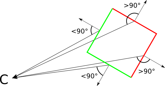
On the other hand, the presence of equally oriented two-sided triangles allows us to specify what is “inside” and “outside” of a closed object. By definition, we should not see the inner parts of a closed object. This means that for any closed object, regardless of the location of the camera, the front faces completely overlap the rear .

Which in turn means that we don’t need to draw the back faces at all, because they will still be redrawn by the front faces!

Triangles classification

Let's formalize and implement it. Suppose we have a triangle normal vector$$→ N and vector$\vec{N}$$$→ V from the top of the triangle to the camera.$\vec{V}$ Let be $$→ N points outside the object. To classify a triangle as a front or back, we calculate the angle between$\vec{N}$$$$\vec{N}$ and $$→ V , then check if they are in$\vec{V}$$$90 ∘ relative to each other. We can again use the properties of the scalar product to further simplify it. Do not forget that if we denote by$90^\circ$

$$ a l p h a angle between$\ alpha$$$$\vec{N}$ and $$$\vec{V}$ then

$$

$${{\langle \vec{N}, \vec{V} \rangle} \over {|\vec{N}||\vec{V}|}} = cos(\alpha)$$

Insofar as $$c o s ( α ) is non-negative with$cos(\alpha)$$$| α | ≤ 90 ∘ , to classify a face as an anterior or posterior we only need to know its sign. It is worth noting that$|\alpha| \le 90^\circ$$$$|\vec{N}|$ and $$| → V | always positive, so they do not affect the sign of the expression.$|\vec{V}|$ Consequently

$$

$$sign(\langle \vec{N}, \vec{V} \rangle) = sign(cos(\alpha))$$

That is, the classification will be very simple:

$$$\langle \vec{N}, \vec{V} \rangle \le 0$	Back side
$$$\langle \vec{N}, \vec{V} \rangle > 0$	Front face

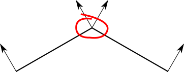
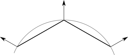
Border case $$⟨ → N , → V ⟩ = 0 corresponds to the case in which we see the edge of the triangle, that is when the camera and triangle coplanar (coplanar). We can classify it in any way, and this will not greatly affect the result, so we decide to classify it as a back face in order to avoid processing degenerate triangles. Where do we get the normal vector? It turns out that there is a vector operation - avector product$\langle \vec{N}, \vec{V} \rangle = 0$

$$→ A × → B , receiving two vectors$\vec{A} \times \vec{B}$$$$\vec{A}$ and $$→ B and the resulting perpendicular vector. We can easily get two vectors, coplanar to a triangle, subtracting its vertices from each other, that is, calculating the direction of the triangle normal vector$\vec{B}$$$A B C will be a simple operation:$ABC$

$$

$$\vec{V_1} = B - A$$

$$

$$\vec{V_2} = C - A$$

$$

$$\vec{P} = \vec{V_1} \times \vec{V_2}$$

Notice that I said “the direction of the normal vector” and not “the normal vector”. There are two reasons for this. The first is that$$| → P | not necessarily equal$|\vec{P}|$$$$1$ . This is not very important, because normalization $$→ P is a trivial operation, and because we care only for the sign$\vec{P}$$$$\langle \vec{N}, \vec{V} \rangle$ .

But the second reason is that if $$→ N is the normal vector$\vec{N}$$$A B C , then it is and$ABC$$$$\vec{-N}$ !

Of course, in this case it is very important for us in which direction $$→ N , because this is exactly what allows us to classify triangles as front or rear. And the vector product is not commutative; in particular,$\vec{N}$$$$\vec{A} \times \vec{B} = -\vec{B} \times \vec{A}$ .This means that we cannot simply subtract the vertices of the triangle in any order, because it determines whether the normal indicates "inward" or "outward."

Although the vector product is not commutative, it is not accidental, of course.

The coordinate system that we used all the time (X to the right, Y up, Z forward) is called a left-sided one, because you can direct the thumb, index and middle finger of your left hand in these directions (thumb up, index forward, middle to the right). The right-side coordinate system is similar to it, but the index finger of the right hand points to the left.

Shading

Let's continue to add a "realism" to the scene; In this chapter, we will learn how to add lights to the scene and how to light the objects it contains.

This chapter is called Shading , not Lighting ; these are two closely related, but different concepts. Lighting refers to mathematics and the algorithms needed to calculate the effect of lighting on one point of the scene; Shading uses techniques to propagate the effects of a light source from a discrete set of points on objects as a whole.

In the chapter Lighting section Tracing raysI have already told you everything you need to know about lighting. We can set the ambient, point and directional lighting; the calculation of the illumination of any point in the scene at a given position and surface normal at this point is performed in the same way both in the ray tracer and in the rasterizer; The theory is exactly the same.

The more interesting part that we will study in this chapter is how to take this " illumination at a point " and make it work for objects consisting of triangles.

Flat shading

Let's start with the simple.Since we can calculate the illumination at a point, let's just choose any point in the triangle (say, its center), calculate the illumination there and use the luminance value to shade the entire triangle (to do actual shading we can multiply the color of the triangle by the luminance value):



Not so so bad. And it's very easy to see why it happened. Each point in the triangle has the same normal, and as long as the light source is far enough, the light vectors are approximately parallel, that is, each point receives approximately an equal amount of light. This roughly explains the differences between the two triangles of which each side of the cube consists.

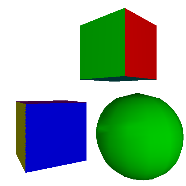
But what happens if we take an object for which each point has its own normal?



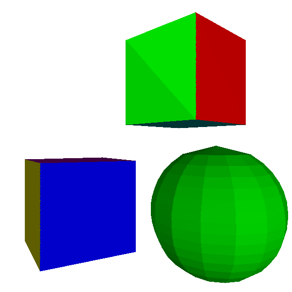
Not very good. Obviously, the object is not a real sphere, but an approximation consisting of flat triangular fragments. Since this type of lighting makes curved objects look flat, it is called flat shading .

Guro Shading

How can we improve the picture? The simplest way for which we already have almost all the tools is to calculate the illumination not of the center of the triangle, but of its three vertices; these lighting values ​​from$$$0.0$ before $$1.0 can then be linearly interpolated first along the edges and then over the surface of the triangle, filling each pixel with a smoothly changing shade. That is, in fact, this is exactly what we did in the chapterRendering of Shaded Triangles; the only difference is that we calculate the brightness values ​​at each vertex using the lighting model, rather than assigning fixed values.This is calledGuro shading by thename of Henri Gouret, who invented this idea in 1971. Here are the results of its application to the cube and sphere: Thecube looks a little better; the unevenness is now gone, because both triangles of each side have two common vertices, and of course the illumination for both of them is calculated exactly the same.$1.0$







However, the sphere still looks faceted, and the irregularities on its surface look very wrong. This should not surprise us, because in the end we work with the sphere as with a set of flat surfaces. In particular, we use very different normals for neighboring faces - and in particular, we calculate the illumination of the same vertex using the very different normals of different triangles!



Let's take a step back. The fact that we use flat triangles to represent a curved object limits our techniques, but not the property of the object itself.

Each vertex in the sphere model corresponds to a point in the sphere, but the triangles they specify are a simple approximation of the surface of the sphere. Therefore, it would be nice if the vertices represent their points of the sphere as precisely as possible - and this means, among other things, that they should use the real normals of the sphere:



However, this does not apply to the cube; even though the triangles have common vertex positions, each face needs to be shaded independently of the others. The vertices of the cube do not have the only “true” normal.

How to solve this dilemma? Easier than it seems.Instead of calculating the normals of the triangles, we will make them part of the model; thus, the object designer can use the normals to describe the curvature of the surface (or its absence). Also, to take into account the case of a cube and other surfaces with flat faces, we will make the vertex normals the property of a vertex in a triangle , and not the vertex itself:

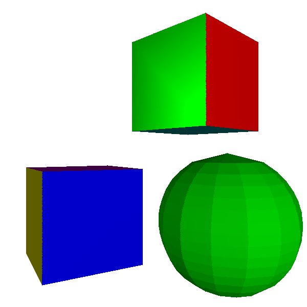
 model { name = cube vertexes { 0 = (-1, -1, -1) 1 = (-1, -1, 1) 2 = (-1, 1, 1) ... } triangles { 0 = { vertexes = [0, 1, 2] normals = [(-1, 0, 0), (-1, 0, 0), (-1, 0, 0)] } ... } } 

Here is a scene rendered using Gouraud shading with appropriate vertex normals: The



cube still looks like a cube, and the sphere now looks much more like a sphere. In fact, looking at its contour, you can determine that it is composed of triangles (this problem can be solved by using more small triangles, spending more computing power).

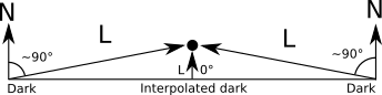
However, illusion collapses when we try to render shiny objects; the mirror light on the sphere is stunningly unrealistic.

There is a smaller problem here: when we shift a point source very close to a large face, we naturally expect it to look brighter, and the effect of specularity will be more pronounced; however, we get a strictly opposite picture:



What is happening here: despite the fact that we expect that points near the center of the triangle will get more light (because $$$\vec{L}$ and $$→ N are approximately parallel), we calculate the illumination not at these points, but at the vertices, the closer the light source is to the surface, thegreater theangle with the normal. This means that each internal pixel will use the brightness interpolated between two low values, that is, they also have a low value:$\vec{N}$

Phong shading

Gourah shading restrictions are easy to overcome, but as usual there is a trade-off between quality and consumed resources.

For flat shading, a single illumination calculation per triangle was used. For Guro shading, three calculations of illumination per triangle plus interpolation of a single attribute (illuminance) over a triangle were required. The next step in this increase in quality and cost per pixel will be the calculation of the illumination for each pixel of the triangle.

This does not seem particularly difficult from a theoretical point of view; after all, we already calculated the illumination for three points, and calculated the pixel-by-pixel illumination for the ray tracer. But the trick here is to figure out where the input data for the light equation come from.

We need $$$\vec{L}$ . With directional light source $$→ L is set. For point light source$\vec{L}$$$→ L is defined as a vector from the point of the scene$\vec{L}$$$P to the position of the light source$P$$$$Q$ . However, we do not have $$Q for each pixel of the triangle, but only for vertices. We have a projection$Q$

$$P - that is$P$$$$x '$ and $$y ′ , which we are going to draw on the canvas! We know that$y '$

$$

$$x' = {Xd \over Z}$$

$$

$$y' = {Yd \over Z}$$

and also we have an interpolated but geometrically correct value for $$oneZ as part of the depth buffering algorithm, therefore$1 \over Z$

$$

$$x' = Xd{1 \over Z}$$

$$

$$y' = Yd{1 \over Z}$$

Therefore, we can get from these values $$$P$ :

$$

$$X = {x' \over d{1 \over Z}}$$

$$

$$Y = {y' \over d{1 \over Z}}$$

$$

$$Z = {1 \over {1 \over Z}}$$

We need $$$\vec{V}$ . This is trivial because we compute $$P as explained above, because the camera position is known. We need$P$

$$$\vec{N}$ .We still have normals only at the vertices. When you have a hammer in your hands, all tasks are like nails , and our hammer is a linear interpolation of attribute values! We can take the values$$$N_x$ , $$$N_y$ and $$N z at each vertex and perceive them as unbound real numbers that can be linearly interpolated. In each pixel, we reassemble the interpolated components into a vector, normalize it, and use it as the normal of this pixel.This technique is calledPhong shadingnamed Bui Tien Phong, who invented it in 1973. Here are its results:The source code and working demo >>The sphere looks great, except for its contour (but the shading algorithm is not to blame for this), and the effect of approaching a light source to a triangle behaves exactly as we expect.This also solves the problem when the source approaches the edge, now we get the expected results:$N_z$













At this stage, we have already reached the capabilities of the ray tracer, developed in the first part, with the exception of shadows and reflections. Here is the output of the rasterizer we are developing when using the same scene:



But the ray-traced version is for reference:



They look almost the same, despite the fact that they use completely different technologies. This is logical, because we used different techniques for rendering the same scene. The only noticeable difference is the edges of the spheres, which the ray tracer renders as mathematically perfect spheres, and the rasterizer approximates as a set of triangles.

Textures

For now, we can render objects such as cubes or spheres and affect them with lighting. But usually we need to render not cubes and spheres, but boxes and planets, game bones or marble.

Consider a wooden box. How to turn a cube into a wooden box? One option is to add a multitude of triangles, creating the structure of the tree, nail heads, and so on. This will work, but because of the geometric complexity of the scene, it will greatly increase, which will affect performance.

Another option is to imitate a box: take the flat surface of the cube and simply draw something resembling wood on top of it. If you do not look at the box, you will never notice the difference.

We will use the second approach. First, we will need an image that we will draw on the surface; in this context, we will call this image a texture , although it is the opposite of what we call the texture of the object - whether it is rough or soft, etc ... Here is the texture of the “wooden box”:


Filter Forge texture - Attribution 2.0 Generic (CC BY 2.0)

Second, we need to specify how the texture should overlap the model. We can set an overlay for each treugog by specifying the texture points applied to each vertex of the triangle:



It is worth noting that you can easily deform the texture or use only parts of the texture by changing the coordinates of the texture for each vertex.

To define this overlay, we use a coordinate system defining the points of this texture; let's call these coordinates$$$u$ and $$v so as not to confuse them with$v$$$$x$$$y , which usually denotes pixels on a canvas. We will also announce that$y$$$$u$ and $$v are real values ​​in the interval$v$$$[ 0 , 1 ] regardless of the resolution of the texture image in pixels. This is very convenient for several reasons; for example, depending on the available RAM capacity, you can use lower or higher resolution textures without changing the model itself. The basic idea of ​​texture mapping is simple: calculate the coordinates$[0, 1]$

$$( U , v ) for each pixel of the triangle, the correspondingtexel(ie,tex-temperatureelement) of texture and paint over that color pixel. Preset pair$(u, v)$$$( u , v ) in texture size$(u, v)$$$( w , h ) superimposed on texel in$(w, h)$$$$(u (w-1), v (h-1))$ .

But we only have coordinates $$$u$ and $$v for three vertices of the triangle, and they are necessary for each pixel ... and probably you already see what should happen. Yes, linear interpolation. We use attribute assignment to interpolate values.$v$$$$u$ and $$v on the side of a triangle that will give us$v$$$( u , v ) in each pixel; we paint the pixel with the appropriate color taken from the texture (perhaps with exposure lighting), and we get ...... mediocre results. The boxes look quite good, but if you look at the diagonal boards, it becomes obvious that they are a bit deformed. What is the mistake? We again fell into the trap of the wrong assumption; we think that$(u, v)$







$$$u$ and $$v along the screen vary linearly. Obviously, this is not the case. Look at the wall of a very long corridor, alternately painted with black and white vertical stripes. When removing the wall, we should see more and more thin stripes. However, if we assume that the coordinate$v$$$u varies linearly with$u$$$x ′ , then it will be wrong:The situation is very similar to the one we encountered in chapterBuffering Depths, and the solution is also very similar: although$x '$



$$$u$ and $$v are non-linear in screen coordinates,$v$$$$u \over z$ and $$vz are linear (Note: the proof of this is very similar to the proof$v \over z$$$onez : assume that${1 \over z}$$$u varies linearly in 3D space, and is replaceable$u$$$$X$ and $$Y on their expression in screen space.). Since we have already interpolated the values$Y$$$onez for each pixel, it is enough to interpolate$1 \over z$$$$u \over z$ and $$vz to get$v \over z$$$$u$ and $$$v$ :

$$

$$u = { {u \over z} \over {1 \over z}}$$

$$

$$v = { {v \over z} \over {1 \over z}}$$

At the same time we will get the expected results:



Source code and working demo >>