Self-oscillations and resonance

Hello!

In connection with questions from readers of my publication [1] regarding the conditions for the excitation of self-oscillations in the mechanical system, I decided to describe the phenomenon of the emergence and maintenance of self-oscillations in detail, highlighting the main areas of the emergence and application of self-oscillations.

In Wikipedia, self-oscillations are explained as follows [2]:

Persistent oscillations in a dissipative dynamic system with nonlinear feedback, supported by constant energy, that is, non-periodic external influence.

Self-oscillations differ from forced oscillations in that the latter are caused by periodic external influences and occur with the frequency of this influence, while the occurrence of self-oscillations and their frequency are determined by the internal properties of the auto-oscillatory system itself. In this case, the frequency becomes almost equal to the resonance.

Auto oscillations in the technique

Self-oscillatory system with a delay (for example, electromechanical bell)
Let's give an example of an electromechanical bell:
')


When the circuit is closed with the button (K), the electromagnet (E) attracts the drummer, the drummer hits the bell and opens the electromagnet's power supply circuit, the contact (T) mechanically connected to it (A) goes back and the process repeats.

When considering the process of self-oscillations, we assume that the force acting on the die (A) of the call changes in proportion to the change in current in the RL circuit.

This assumption is made to simplify consideration, since the dependence of the force on the current in the winding and the gap between the striker and the poles is much more complicated [3].

Below are the design of electromechanical calls and their simplified electrical circuit:



The face varies relative to the set gap according to the relation A * sin (w * t).
Solving the differential equation of the RL chain with initial conditions by a numerical method
for closing and opening the contact, imposing oscillations of the striker on these solutions, we get:

import numpy as np from scipy.integrate import odeint import matplotlib.pyplot as plt R=100;L=0.07;E=100;tm=L/R;T=0.0280;w=2*np.pi/T #  RL     w def dydt(y, t):#  .     return -y/tm def dydt1(y1, t): return -y1/tm+E/L plt.title('   ', size=12) y = odeint(dydt, E/R, np.linspace(0,T/4,300))#  ()   RL, y(0)=E/R plt.plot(np.linspace(0,T/4,300), y,'b',linewidth=2,label=' Fp=Km*Ip')#  y1 = odeint(dydt1, 0, np.linspace(T/2,3*T/4,300))#  ()   RL, y(0)=0 plt.plot( np.linspace(T/2,3*T/4,300), y1,'g',linewidth=2,label=' Fz=Km*Iz') t2=np.linspace(0,T,300) y2=(E/R)*np.sin(w*t2)#    plt.plot(t2, y2,"--r",linewidth=2,label='  ') t3=np.linspace(0,T/4,300) t4=np.linspace(T/2,3*T/4,300) y3=[0 for i in t3] y4=[0 for i in t4] plt.plot(t3, y3,"--k",linewidth=3,label=' Fp   ') plt.plot(t4, y4,"--k",linewidth=3,label=' Fz  ') plt.legend(loc='best') plt.grid(True) plt.show()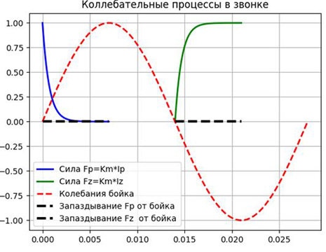 

For an approximate theory, we assume that the force Fτ, expressed by a sequence of rectangular pulses that occurs and disappears instantaneously, but not at the time of the contact, but with a delay τ = L / R. Add Fτ to the graph, we get:

 import numpy as np from scipy.integrate import odeint import matplotlib.pyplot as plt R=100;L=0.07;E=100;tm=L/R;T=0.0280;w=2*np.pi/T #  RL     w def dydt(y, t):#  .     return -y/tm def dydt1(y1, t): return -y1/tm+E/L plt.title('   ', size=12) y = odeint(dydt, E/R, np.linspace(0,T/4,300))#  ()   RL, y(0)=E/R plt.plot(np.linspace(0,T/4,300), y,'b',linewidth=2,label=' Fp=Km*Ip')#  y1 = odeint(dydt1, 0, np.linspace(T/2,3*T/4,300))#  ()   RL, y(0)=0 plt.plot( np.linspace(T/2,3*T/4,300), y1,'g',linewidth=2,label=' Fz=Km*Iz') t2=np.linspace(0,T,300) y2=(E/R)*np.sin(w*t2)#    plt.plot(t2, y2,"--r",linewidth=2,label='  ') def con_n(f): z=0 if np.sin(0)<=np.sin(f)<np.sin(T/4): z=E/R elif np.sin(T/4)<= np.sin(f)<np.sin(3*T/4): z=0 elif np.sin(3*T/4)<=np.sin(f)<np.sin(T+tm): z=E/R return z y3=[con_n(q) for q in t2] plt.plot(t2, y3,"k",linewidth=3,label='  ') plt.legend(loc='best') plt.grid(True) plt.show()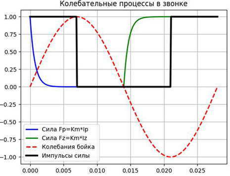 

Let us denote the amplitude of the force Fτ by Aτ, we obtain the expansions of this force in a Fourier series [4] (given that x = a ∙ sin (ω ω t)) for the first two members of the series:



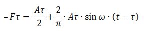
We assume that the constant component of the force Aτ / 2 is compensated by the adjustment.
Then the equation for vibrations of the striker, taking into account its reduced mass m, friction r and flexural rigidity k, takes the form:

(one)

We divide both parts by the weight of the striker, we introduce the notation, we will receive:

(2)

In order to obtain analytical relations for the frequency and amplitude of oscillations of the striker, we solve (2) using the approximate method [5]. Convert (2) to the form:

(3)

Substituting in (3) provided:
skipping the intermediate calculations, we obtain relations for the frequency and amplitude of self-oscillations:



Based on the above relations, it can be concluded that, in the absence of self-induction, the call cannot work, since there is no delay τ = 0 for L = 0. Thus, with zero delay, self-oscillations are not possible.

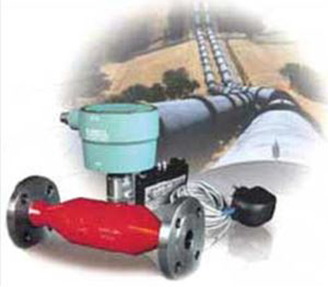
Self-oscillations in the measurement technology (for example, the mechanical resonator of vibration density meters)

Mechanical resonators in the form of tube plates or cylinders are widely used in vibration densitometers, the appearance of which is shown in the figures:





We will consider a resonator with lumped equivalent parameters: mass stiffness and friction characterized by a coefficient

Such a replacement is quite acceptable in a limited frequency range, provided that the natural frequencies of the oscillations of both systems are equal, as well as the energy losses and the attenuation caused by them are equal.

We write the system of equations describing the motion of a resonator in a closed excitation system:



where: F is the effect of the excitation system on the resonator;
D (x) is an unknown feedback operator to be defined; Fupr - the elastic restoring force of the resonator, which in the general case can be described by a nonlinear function; x is the transverse displacement of equivalent mass.

We use the expression of the cubic elastic characteristics of the resonator:



where γ is the coefficient characterizing the deviation of the real elastic characteristic from the linear one.

We transform the written system of equality to the form:



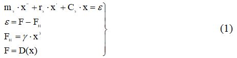
Where - nonlinear component of the elastic force.

The block diagram of the self-oscillatory system, whose work is characterized by equations, (1) is shown in the figure:



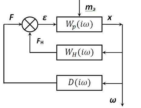
The scheme contains a nonlinear link that performs the function of correcting feedback for a linear resonator having a frequency response:



To solve the problem of synthesizing an optimal excitation system, we use the method of harmonic linearization [6].

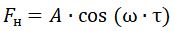
Mechanical resonators are high-quality oscillatory systems that can be considered as narrow-band filters with an output signal of the form: x ~ A ∙ cos ⁡ (ω ∙ τ), where A is the oscillation amplitude of the resonator; ω is the oscillation frequency close to the resonance [7].

Therefore, for a nonlinear element, the following relation holds:



Neglecting the third harmonic filtered by the linear part of the resonator, the frequency response of the linearized link of the nonlinear elasticity of the mechanical resonator can be in the form:



Consider the equation for the first harmonic of oscillations of a linearized system:



To determine the type of the frequency characteristic D (iω), which ensures the compatibility of this system, we exclude intermediate variables by direct substitution of their expressions in terms of other variables. As a result, we get:



From relation (2), we determine the phase shift carried out by the excitation system:



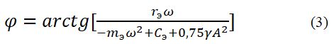
It is easy to establish that the frequency of self-oscillations will not depend on friction when the phase shift φ = π / 2, then:



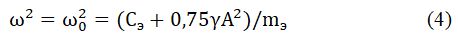
Under this condition, it follows from (2) that the excitation system must be the differentiating link D (iω) = (i * re e ω), i.e.



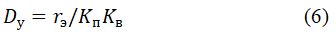
From (5) it follows that the frequency response of the feedback circuit of the excitation system should be proportional to the coefficient of friction

The excitation system consists of three elements, D (iω) = D * D * D (), which characterize the frequency characteristics: receiver D, amplifier D and pathogen D () of oscillations. The receiver is differentiating - D = K * i * ω , and the pathogen is amplifying
link - Dv = Kv.

To fulfill condition (5), the amplifier must have a frequency response:



The gain should change with the change in friction.
A link with a variable gain can be realized with the simplest non-linearity of the type of a two-position relay, which has a frequency characteristic of the first harmonic [6]:



Where 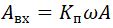- the amplitude of the first harmonic at the input of the amplifier; - the output voltage of the amplifier supplied to the exciter.

From (6) and (7) one can get an expression for the amplitude of steady self-oscillations of the resonator:



To eliminate this amplitude effect on the resonator frequency, it is possible to stabilize the amplitude A by varying the voltage U0 with a regulator that stabilizes the amplitude of the input signal ABi coming from the oscillation receiver.

From the above we can conclude that the frequency of self-oscillations of the resonator of the vibration measuring transducer will not depend on friction during phase shift φ = π / 2, when the excitation system is a differentiating element, and will not depend on the amplitude of self-oscillations when the input signal of this link stabilizes.

Self-oscillations in radio generators (for example, solving an equation
Van der Pol

A generalized diagram of the radio oscillator self-oscillations is shown in the figure:



The mechanism of excitation of self-oscillations in the generator can be qualitatively described as follows. Even in the absence of voltage at the output of the amplifier, the voltage in the circuit experiences random fluctuations. They are amplified by the amplifier and re-enter the circuit through the feedback circuit.

In this case, the component at the natural frequency of the high-quality contour will be separated from the noise spectrum of fluctuations. If the energy introduced into the circuit in this way exceeds the energy of the losses, the amplitude of oscillations increases.

The main model describing the self-oscillations in a radio-technical generator is the Van der Pol equation. We give the van der Pol equation to a form containing a single control parameter with dimensionless variables:



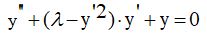
We obtain phase portraits (left) and temporal realizations of oscillations (right) of the van der Pol oscillator: λ = 0.1, λ = 1.1

 import numpy as np from scipy.integrate import odeint import matplotlib.pyplot as plt def f(y, x): y1, y2 = y return [y2,(0.1-y2**2)*y2-y1] x= np.linspace(0,200,601) y0 = [0.0001,0.0001] [y1,y2]=odeint(f, y0, x).T plt.subplot(221) plt .plot(y1,y2,linewidth=2) plt .grid(True) plt.subplot(222) plt .plot(x,y1,linewidth=2, label=' \n ') plt.legend(loc='best') plt .grid(True) def f_1(y, x): y1, y2 = y return [y2,(1.1-y2**2)*y2-y1] x= np.linspace(0,200,601) y0 = [0.0001,0.0001] [y1,y2]=odeint(f_1, y0, x).T plt.subplot(223) plt .plot(y1,y2,linewidth=2) plt .grid(True) plt.subplot(224) plt .plot(x,y1,linewidth=2, label=' \n ') plt.legend(loc='best') plt .grid(True) plt.show() 

For λ = 10.0

 import numpy as np from scipy.integrate import odeint import matplotlib.pyplot as plt def f(y, x): y1, y2 = y return [y2,(10.0-y2**2)*y2-y1] x= np.linspace(0,200,601) y0 = [0.0001,0.0001] [y1,y2]=odeint(f, y0, x).T plt.subplot(221) plt .plot(y1,y2,linewidth=2) plt .grid(True) plt.subplot(222) plt .plot(x,y1,linewidth=2, label=' \n ') plt.legend(loc='best') plt .grid(True) plt.show() 

The van der Pol equation has a single singular point. which is a stable node when steady focus when unstable focus when and unstable node when . If the self-excitation condition is fulfilled, there is also a limit cycle on the phase plane corresponding to the periodic self-oscillation mode.

Chemical fluctuations. Brusselator

An important and nontrivial example of self-oscillatory processes are certain chemical reactions. Chemical fluctuations are fluctuations in the concentrations of reactants.

To date, quite a lot of vibrational reactions are known. The most famous of them was discovered by B.P. Belousov in 1950 and later studied in detail by A.M. Zhabotinsky. The Belousov-Zhabotinsky (BZ) reaction is the process of oxidation of malonic acid when interacting in the presence of ions as a catalyst.

During the reaction, the solution periodically changes its color: blue - red - blue - red, etc. In addition to simple periodic oscillations, the BZ reaction demonstrates (depending on the experimental conditions) a variety of different types of space-time dynamics, which have not yet been completely investigated.

Various mathematical models of the reaction of the BZ have been proposed (for example, the Field, Keres and Noyes models are “oregonator”), but none of them fully describes all the details observed in the experiment.

We consider a simpler model example: a hypothetical chemical reaction, called the Brusselator [8]. The equations of this reaction are:



It is assumed that the reagents A and B are in excess, so that their concentrations can be considered constant, and D and E do not enter into any reactions. Let us compose kinetic equations corresponding to the reaction, which describe the dynamics of the concentrations of the reacting substances.

Since the number of chemical reaction acts per unit time is determined by the probability of collision of reactant molecules, the rates of change in the concentrations of the reaction products are proportional to the product of the concentrations of the corresponding reactants with proportionality coefficients, called reaction rate constants. Then the kinetic equations can be written in the form:



The symbols Y, X will now denote the corresponding concentrations. Note that it follows from the third equation of the system that the rate of formation of substance X depends on its concentration, i.e. This stage of the reaction is autocatalytic. We present equations (1) to a dimensionless form, containing the minimum number of control parameters. To do this, go to the new variables, Then equations (1) take the form:



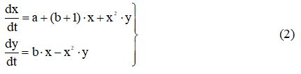
Construct phase portraits for: a = 1.0; b = 2.1; b = 3.0; b = 5.0

 import numpy as np from scipy.integrate import odeint import matplotlib.pyplot as plt b=2.1 def f(y, x): y1, y2 = y return [1-(b+1)*y1+(y1**2)*y2, b*y1-(y1**2)*y2] x= np.linspace(0,100,1001) y0 = [0.5,1.5] [y1,y2]=odeint(f, y0, x).T plt .plot(y1,y2,linewidth=2,label='a=1.0, b=%s'%b) plt.legend(loc='best') plt .grid(True) plt.show()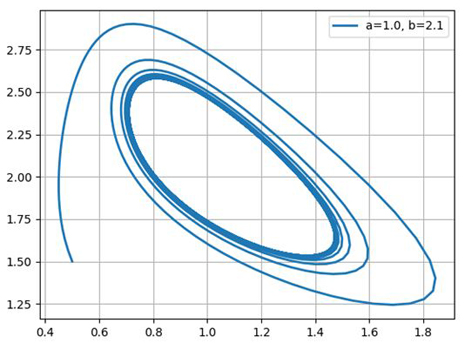 

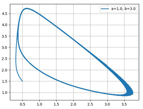
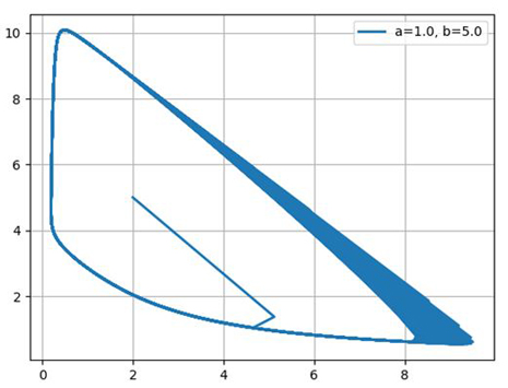
Thus, a chemical oscillator exhibits a behavior typical of self-oscillatory systems and quite similar, for example, to the van der Pol oscillator.

Autooscillations in biosystems (using the example of the Lotka Volterra model - “Predator is a victim”)

In the dynamics of populations there are many examples when the change in the number of populations over time is oscillatory. One of the most famous examples of the description of the dynamics of interacting populations are the Volterra – Lotk equations.

Consider the model of the interaction of predators and their prey, when there is no rivalry between individuals of one species. Let x and y be the number of preys and predators, respectively. Suppose that the relative increase in prey y '/ x is a-by, a> 0, b> 0, where a is the reproduction rate of prey in the absence of predators, and -by is the loss from predators.

The development of a predator population depends on the amount of food (prey), in the absence of food (x = 0) the relative rate of change of the predator population is y '/ y = -c, c> 0, the presence of food compensates for a decrease, and for x> 0 we have y' / y = (- c + d * x), d> 0.

Thus, the Volterra — Lotka system has the form:



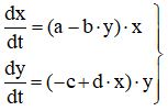
where a, b, c, d> 0.

Consider the phase portrait of the Volterra Lotka system, for a = 4 b = 2.5, c = 2, d = 1 and graphs of its solution with the initial condition x (0) = 3, y (0) = 1, constructed by the Python program for the numerical solution of the system ordinary differential equations:

 import numpy as np from scipy.integrate import odeint import matplotlib.pyplot as plt a=4;b=2.5; c=2; d=1 def f(y, t): y1, y2 = y return [y1*(ab*y2),y2*( -c+d*y1)] t = np.linspace(0,10,201) y0 = [3, 1] [y1,y2]=odeint(f, y0, t).T plt.figure() plt .plot(y1,y2,linewidth=2) plt .grid(True) plt.figure() plt .plot(t,y1,linewidth=2) plt .plot(t,y2,linewidth=2) plt .grid(True) plt.show()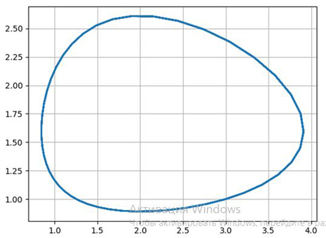 

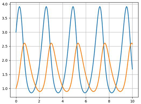
It is seen that the process has an oscillatory nature. With a given initial ratio of the number of individuals of both species 3: 1, both populations first grow. When the number of predators reaches a value of b = 2.5, the population of victims does not have time to recover and the number of victims begins to decrease.

The decrease in the amount of food after a while begins to affect the predator population, and when the number of prey reaches x = c / d = 2 (at this point y '= 0), the number of predators also begins to decrease along with the reduction in the number of prey. Reduction of populations occurs until the number of predators reaches the value y = a / b = 1.6 (at this point x '= 0).

From this point on, the prey population begins to grow, after a while food becomes sufficient to ensure the growth of predators, both populations grow, and ... the process repeats again and again.

The considered model can describe the behavior of competing firms, population growth, the number of warring armies, changes in the environmental situation, the development of science, etc.

Thanks for attention!!!

References:

1. A mathematical model of a vibrating level gauge with a resonator in the form of a cantilever elliptical tube.
2. Auto-oscillations
3. The basic equations of the problem of the synthesis of a w-shaped electromagnet.
4. On the classification of Fourier transform methods by examples of their software implementation by means of Python.
5. Theodorchik K.F. Self-oscillating systems. GITL., 1952, 272 p.
6. The method of harmonic linearization by means of Python.
7. Zhukov Yu.P. Vibration density meter. - M. Energoatomizdat, 1991. -
144c: il. - (B-ka on automation; Vol. 678)
8. I. Prigogine, R. Lefebvre Brusselator M. Science, 1968