This article is divided into two main parts, Ray Tracing and Rasterization , which discuss two main ways to get beautiful images from data. The General Concepts chapter presents some basic concepts necessary for understanding these two parts.

In this paper, we will focus not on speed, but on a clear explanation of the concepts. The code of examples is written in the most understandable way, which is not necessarily the most efficient for the implementation of algorithms. There are many ways to implement, I chose the one that is easiest to understand.
')
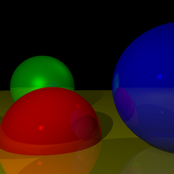
The “end result” of this work will be two complete, fully working renderers: a ray tracer and a rasterizer. Although they use very different approaches, they render similar results when rendering a simple scene:



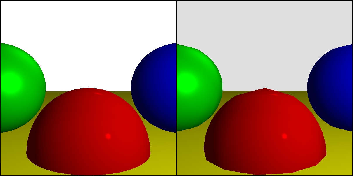
Although their capabilities largely overlap, they are not similar, so the article discusses their strengths:



The article in the form of an informal pseudocode presents the code of examples, it also contains fully working implementations, written in JavaScript, rendered on the canvas element, which can be run in the browser.

Why read this article?

This work will give you all the information you need to write software renderers. Although in our era of video processors few will find compelling reasons for writing a purely software renderer, writing experience will be valuable for the following reasons:

1. Shaders In the first video processors, the algorithms were hard-coded in hardware, but in modern programs the programmer must write his own shaders. In other words, you still need to implement large fragments of the rendering software, only now it is executed in the video processor.
2. Understanding . Regardless of whether you use a ready-made pipeline or write your shaders, understanding what happens behind the scenes will allow you to make better use of the finished pipeline and write shaders better.
3. Interesting . Few areas of computer science can boast the ability to instantly obtain visible results, which gives us computer graphics. The feeling of pride after starting the execution of the first SQL query is incomparable with the fact that you feel the first time when you manage to trace reflections correctly. I taught computer graphics at the university for five years. I was often amazed how I managed to enjoy semester after semester: in the end, my efforts justified themselves with the students' joy that they could use their first renders as desktop wallpapers.

General concepts

Canvas

In the process, we will draw objects on the canvas . Canvas is a rectangular array of pixels that can be individually painted. Will it be displayed on the screen, printed on paper, or used as a texture for subsequent rendering? This is not important for our work: we will focus on rendering images on this abstract rectangular array of pixels.

Everything in this article we will build from a simple primitive: draw a pixel on the canvas with the specified color:

  canvas.PutPixel (x, y, color) 

Now we will study the parameters of this method - coordinates and colors.

Coordinate systems

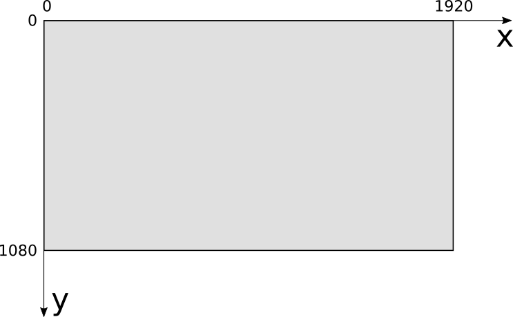
The canvas has a certain width and height in pixels, which we call $$$C_w$ and $$$C_h$ . To work with its pixels, you can use any coordinate system. On most computer screens, the origin point is in the upper left corner. $$$x$ increases to the right as well $$$y$ - way down:



This is a very natural coordinate system taking into account the organization of video memory, but for people it is not very familiar. Instead, we will use the coordinate system commonly used for drawing graphs on paper: the origin of coordinates in the center $$$x$ increases to the right as well $$$y$ - up:



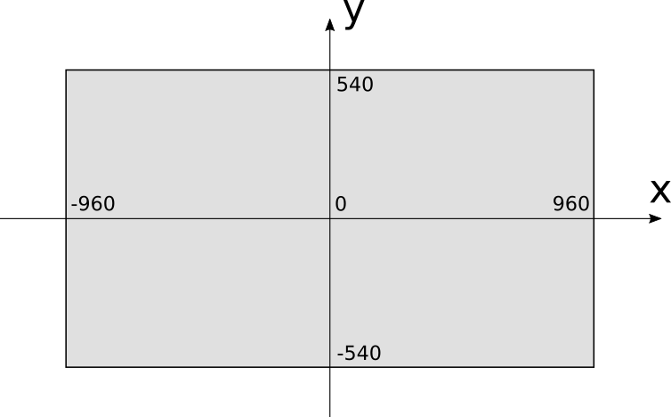
When using this coordinate system, the coordinate $$$x$ is in the interval $$$[{- C_w \ over 2}, {C_w \ over 2}]$ and coordinate $$$y$ - in the interval $$$[{- C_h \ over 2}, {C_h \ over 2}]$ (Note: strictly speaking, or $$${- C_h \ over 2}$ , or $$${C_h \ over 2}$ are outside the interval, but we will ignore it.). For simplicity, when trying to work with pixels outside of a possible interval, nothing will just happen.

In the examples, the canvas will be drawn on the screen, so it is necessary to perform transformations from one coordinate system to another. If we assume that the screen is the same size as the canvas, then the transformation equations will be simple:

$$

$$S_x = {C_w \ over 2} + C_x$$

$$

$$S_y = {C_h \ over 2} - C_y$$

Color models

The theory of the color work itself is amazing, but, unfortunately, is beyond the scope of our article. Below is a simplified version of those aspects that are important to us.

Color is the way in which the brain interprets photons that enter our eye. These photons carry energy of different frequencies, our eyes associate these frequencies with colors. The smallest energy perceived by us has a frequency of about 450 THz, we perceive it as red. At the other end of the spectrum are 750 THz, which we see as "purple." Between these two frequencies, we see a continuous spectrum of colors (for example, green is about 575 THz).

In the normal state, we cannot see frequencies outside this range. Higher frequencies carry more energy, so infrared radiation (frequencies below 450 THz) is harmless, but ultraviolet (frequencies above 750 THz) can burn the skin.

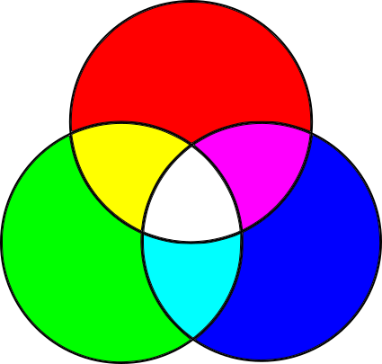
Any color can be described as various combinations of these colors (in particular, “white” is the sum of all colors, and “black” is the absence of all colors). Describing the colors with the exact frequency is inconvenient. Fortunately, you can create almost all colors as a linear combination of all three colors, which we call "primary colors."

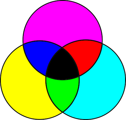
Subtractive color model

Objects have a different color because they absorb and reflect light in different ways. Let's start with white light, such as solar light (Note: sunlight is not completely white, but for our purposes it is close enough to it.). White light contains frequencies of all colors. When light falls on an object, depending on the material of the object, its surface absorbs some of the frequencies and reflects the rest. Part of the reflected light enters our eye and the brain transforms it into color. What color? In the sum of all reflected frequencies (Note: due to the laws of thermodynamics, the rest of the energy is not lost, it basically turns into heat.).

To summarize: we start with all the frequencies, and subtract some amount of primary colors to create a different color. Since we subtract frequencies, such a model is called a subtractive color model .

However, this model is not entirely correct. In fact, the main colors in the subtractive model are not blue, red and yellow, as taught by children and students, but cyan (Cyan), magenta (Magenta) and yellow (Yellow). Moreover, the mixture of the three primary colors gives some darkish color, which does not quite look like black, so black is added as the fourth “primary” color. Black is denoted by the letter K - and so it turns out the CMYK color model used for printers.

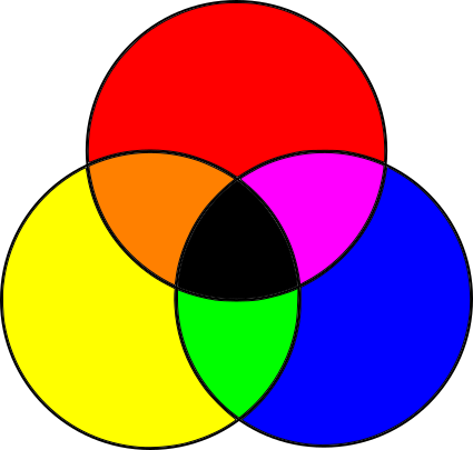
Additive color model

But this is only half the story. The screens of the monitors are opposite to the paper. The paper does not emit light, but simply reflects part of the light falling on it. On the other hand, the screens are black, but they emit light. On paper, we started with white light and subtracted unnecessary frequencies; on the screen, we start with a lack of light and add the necessary frequencies.

It turns out that this requires other primary colors. Most colors can be created by adding different sizes of red, green and blue to the black surface; This is an RGB color model, an additive color model :

Forget about the details

Now that you know all this, you can selectively forget unnecessary details and focus on what is important for work.

Most colors can be represented in RGB or CMYK (or in many other color models) and can be converted from one color space to another. Since our main task is to render images to the screen, we will use the RGB color model.

As stated above, objects absorb a portion of the light falling on them, and reflect the rest. We perceive the absorbed and reflected frequencies as the “color” of the surface. From now on, we will perceive color simply as a property of the surface and forget about the frequencies of the absorbed light.

Depth and color representation

As explained in the previous section, monitors can create colors from various combinations of red, green, and blue.

How different can their brightness be? Although voltage is a continuous variable, we will process colors using a computer using discrete values. The more different shades of red, green and blue we can set, the more colors we can create.

The most popular format today uses 8 bits per primary color (also called a color channel ). 8 bits per channel gives us 24 bits per pixel, that is, the total $$$2 ^ {24}$ various colors (approximately 16.7 million). This format, known as 888, will be used in our work. We can say that this format has a color depth of 24 bits.

However, it is by no means the only possible format. Not so long ago, 15-bit and 16-bit formats were used to save memory, assigning 5 bits per channel or 5 bits for red, 6 for green, and 5 for blue (this format was known as 565). Why did green get an extra bit? Because our eyes are more sensitive to changes in green than red or blue.

16 bits give us $$$2 ^ {16}$ flowers (about 65 thousand). This means that we get one color for every 256 colors of the 24-bit mode. Although 65,000 is a lot, on images with gradually changing colors, you can notice very small “steps” that are invisible in 16.7 million colors, because there are enough bits to represent intermediate colors. 16.7 million colors are more and more than the human eye can recognize, so in the foreseeable future we will most likely continue to use 24-bit colors. (Note: this only applies to displaying images, storing images with a wider range is a completely different matter, which we will look at in the Lighting chapter.)

To represent the color, we will use three bytes, each of which will contain the value of an 8-bit color channel. In the text, we denote colors as $$$(R, G, B)$ - eg, $$$(255, 0, 0)$ - it is pure red color; $$$(255, 255, 255)$ - white, and $$$(255, 0, 128)$ - reddish purple.

Color management

For color management, we use several operations (Note: if you know linear algebra, then perceive colors as vectors in three-dimensional color space. In the article I will introduce you to the operations that we will use for readers unfamiliar with linear algebra.).

We can increase the color brightness by increasing each color channel by a constant:

$$

$$k (R, G, B) = (kR, kG, kB)$$

We can add two colors together by adding color channels separately:

$$

$$(R_1, G_1, B_1) + (R_2, G_2, B_2) = (R_1 + R_2, G_1 + G_2, B_1 + B_2)$$

For example, if we have a reddish purple

$$

$$(252, 0, 66)$$

and we want to get exactly the same shade, but three times less bright, then we multiply each channel by $$$1 \ over 3$ and get $$$(84, 0, 22)$ . If we want to combine red $$$(255, 0, 0)$ and green $$$(0, 255, 0)$ then we fold the channels and get $$$(255, 255, 0)$ that is, yellow.

An attentive reader may say that with such operations we may get incorrect values: for example, doubling the brightness $$$(192, 64, 32)$ , we get the value of R outside the color range. We will assume that any value greater than 255 is equal to 255, and any value less than 0 is equal to 0. This is more or less the same as when you take a picture with a too slow or slow shutter speed - completely black or completely white areas appear on it.

Scene

Canvas (canvas) is an abstraction on which we render everything. What do we render? Another abstraction is a scene .

A scene is a collection of objects that you need to render. It can be anything from a single sphere hanging in empty space (we start with this one) to an incredibly detailed model of the insides of the nose of the ogre.

In order to talk about objects in the scene, we need a coordinate system. You can choose any, but we will find something useful for our purposes. Y axis will be pointing up. X and Z axes are horizontal. That is, the XZ plane will be “floor”, and XY and YZ will be vertical “walls”.

Since we are talking here about “physical” objects, we need to select the units of their measurement. They can also be any, but they strongly depend on what is represented in the scene. “1” can be one millimeter when modeling a circle, or one astronomical unit when modeling a solar system. Fortunately, nothing described below depends on the units of measurement, so we will simply ignore them. As long as we maintain uniformity (that is, “1” always means the same thing for the whole scene), everything will work fine.

Part I: ray tracing

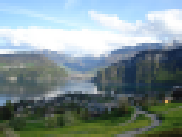
Imagine that you are in some exotic place and enjoy a stunning view, so stunning that you just have to capture it in the picture.


Swiss landscape

You have paper and markers, but absolutely no artistic talent. Is all lost?

Not necessary. Maybe you have no talent, but there is a method.

You can do the most obvious thing: take an insect screen and place it in a rectangular frame, attaching the frame to a stick. Then look at the landscape through this grid, select the best angle and place another stick exactly where the head should be in order to get the exact same point of view:

You have not started drawing yet, but at least you have a fixed point of view and a fixed frame through which you see the landscape. Moreover, this fixed frame is divided into small squares. And now we proceed to the methodical part. Draw a grid on paper with the same number of squares as in the insect screen. Now look at the upper left square of the grid. What color is dominant in it? Sky blue. Therefore, we draw in the upper left square of the paper sky-blue color. Repeat the same for each square and pretty soon we will get a pretty good picture of the landscape, as if visible from the window:


Rough terrain approximation

If you think about it, the computer, in essence, is a very methodical machine that has absolutely no artistic talents. If we replace the squares on paper with pixels on the screen, we can describe the process of rendering the scene as follows:

  For each pixel of the canvas
     Color it with the desired color 

Very simple!

However, such code is too abstract to be implemented directly in the computer. Therefore, we can go into the details a bit:

  Place the eye and frame in the right places.
 For each pixel of the canvas
     Determine the grid square corresponding to this pixel.
     Determine the color visible through this square.
     Fill pixel with this color 

This is still too abstract, but it is already beginning to sound like an algorithm. Surprisingly, this is the high-level description of the entire ray tracing algorithm. Yes, everything is so simple.

Of course, the devil is in the details. In the following chapters we will take a closer look at all these stages.

Ray Tracing Basics

One of the most interesting things in computer graphics (and perhaps the most interesting) is drawing graphics on the screen. In order to proceed to it as soon as possible, we will first make some minor simplifications in order to display something on the screen right now . Of course, such simplifications imply some limitations on our possible actions, but in subsequent chapters we will step by step get rid of these limitations.

First, we will assume that the viewpoint is fixed. The viewpoint is the place where the eye is located in our analogy, and it is usually called the camera position ; let's call him $$$O = (O_x, O_y, O_z)$ . We will assume that the camera is located at the origin of the coordinate system, i.e. $$$O = (0, 0, 0)$ .

Secondly, we will assume that the orientation of the camera is also fixed, that is, the camera is always directed to the same place. We assume that it is looking down the positive Z axis, the positive Y axis is pointing up, and the positive X axis is right:



The position and orientation of the camera is now fixed. But we still do not have a “framework” from the analogy proposed by us, through which we look at the scene. We assume that the frame has dimensions $$$V_w$ and $$$V_h$ it is frontal with respect to the position of the camera (i.e., perpendicular $$$\ vec {Z _ +}$ ) and is at a distance $$$d$ its sides are parallel to the X and Y axes, and it is centered relative to $$$\ vec {Z _ +}$ . The description looks complicated, but in fact everything is quite simple:



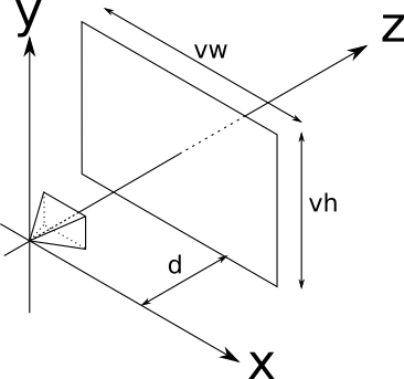
This rectangle, which will be our window to the world, is called the viewport . In essence, we will draw on the canvas all that we see through the viewing window. It is important that the size of the viewport and the distance to the camera determine the angle of visibility from the camera, called the field of view or FOV for short. In people, the horizontal FOV is almost $$$180 ^ \ circ$ however, most of it is vague peripheral vision without a sense of depth. In general, reliable images are obtained using FOV $$60  c i r c in the vertical and horizontal direction; this can be achieved by setting$60 ^ \ circ$$$$V_w = V_h = d = 1$ .

Let's go back to the “algorithm” presented in the previous section, we denote its steps by numbers:

 Place the eye and frame in the right places (1)
For each pixel of the canvas
    Determine the grid square corresponding to this pixel (2)
    Determine the color visible through this square (3)
    Fill pixel with this color (4) 

We have already completed step 1 (or, more precisely, got rid of it for a while). Step 4 is trivial ( canvas.PutPixel(x, y, color)). Let's take a quick look at step 2, and then focus on much more complicated ways to implement step 3.

From canvas to viewport

In step 2, we need to " Determine the grid square corresponding to this pixel ." We know the coordinates of the pixel on the canvas (we draw them all) - let's call them$$$C_x$ and $$$C_y$ .Notice how conveniently we positioned the viewing window - its axes correspond to the orientation of the axes of the canvas, and its center corresponds to the center of the viewing window. That is, you can move from the coordinates of the canvas to the coordinates of space by simply changing the scale!

$$

$$V_x = C_x {V_w \over C_w}$$

$$

$$V_y = C_y {V_h \over C_h}$$

There is another subtlety. Although the viewport is two-dimensional, it is built into three-dimensional space. We indicated that it is at a distance d from the camera. At each point in this plane (called the projection plane ), by definition$$$z = d$ . Consequently,

$$

$$V_z = d$$

And on this we have completed step 2. For each pixel $$( C x , C y ) of the canvas we can define the corresponding point of the viewport$(C_x, C_y)$$$$(V_x, V_y, V_z)$ . In step 3, we need to determine what color the light passes through. $$( V x , V y , V z ) in terms of camera view$(V_x, V_y, V_z)$$$$(O_x, O_y, O_z)$ .

Trace the rays

So through what color does light reach $$( O x , O y , O z ) after passing through$(O_x, O_y, O_z)$$$$(V_x, V_y, V_z)$ ?

In the real world, light emanates from a source of light (the sun, light bulbs, etc.), reflects from several objects, and finally reaches our eyes. We can try to simulate the path of each photon emitted from simulated light sources, but it will be incredibly time consuming (Note: the results will be amazing. This technique is called photon tracing or photon distribution; unfortunately, it is not related to the topic of our article.) . We would not only have to simulate millions and millions of photons, but after passing through the viewing window$$( O x , O y , O z ) would reach only a small part of them. Instead, we will trace the rays "in the reverse order" - we will start with the beam on the camera, passing through a point in the viewing window and moving until it collides with some object in the scene. This object will be “visible” from the camera through this point of the viewport. That is, as a first approximation, we simply take the color of this object as “the color of light that has passed through this point”. Now we just need a few equations.$(O_x, O_y, O_z)$

Ray equation

The best way to represent rays for our purpose would be to use a parametric equation. We know that the beam passes through O, and we know its direction (from O to V), so we can express any point P of the beam as

$$

$$P = O + t(V - O)$$

where t is an arbitrary real number.

Let's denote$$( V - O ) , that is, the direction of the beam, as$(V - O)$$$$\vec{D}$ ; then the equation takes the simple form

$$

$$P = O + t\vec{D}$$

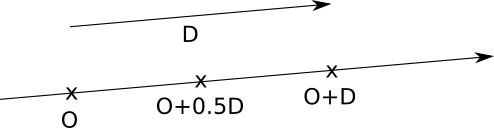
You can read more about this in linear algebra; it is intuitively clear that if we start from the starting point and move forward to some multiple of the direction of the beam, we will always move along the beam:

Sphere equation

Now we need to add some objects to the scene so that the rays can collide with something . We can choose any arbitrary geometric primitive as a building block of scenes; for ray tracing the simplest primitive for mathematical manipulations will be the sphere.

What is a sphere? A sphere is a set of points lying at a constant distance (called the sphere’s radius ) from a fixed point (called the center of the sphere):



Notice that judging by definition, the spheres are hollow.

If C is the center of the sphere, and r is the radius of the sphere, then the points P on the surface of the sphere satisfy the following equation:

$$

$$distance(P, C) = r$$

Let's experiment a bit with this equation. The distance between P and C is the length of the vector from P to C:

$$

$$|P - C| = r$$

The length of a vector is the square root of its scalar product itself:

$$

$$\sqrt{\langle P - C, P - C \rangle} = r$$

And to get rid of the square root,

$$

$$\langle P - C, P - C \rangle = r^2$$

Ray meets the sphere

Now we have two equations, one of which describes the points of the sphere, and the other the points of the ray:

$$

$$\langle P - C, P - C \rangle = r^2$$

$$

$$P = O + t\vec{D}$$

The point P, in which the beam falls on a sphere, is both a point of the beam and a point on the surface of the sphere, so it must satisfy both equations at the same time. Notice that the only variable in these equations is the parameter t, because O,$$→ D , C, and r are given, and P is the point we need to find. Since P is the same point in both equations, we can replace P in the first by the expression for P in the second. It gives us$\vec{D}$

$$

$$\langle O + t\vec{D} - C, O + t\vec{D} - C \rangle = r^2$$

What values ​​of t satisfy this equation?

In its current form, the equation is rather cumbersome. Let's transform it to see what can be obtained from it.

First, we denote$$$\vec{OC} = O - C$ . Then the equation can be written as

$$

$$\langle \vec{OC} + t\vec{D}, \vec{OC} + t\vec{D} \rangle = r^2$$

Then we decompose the scalar product into its components, taking advantage of its distributivity:

$$

$$\langle \vec{OC} + t\vec{D}, \vec{OC} \rangle + \langle \vec{OC} + t\vec{D}, t\vec{D} \rangle = r^2$$

$$

$$\langle \vec{OC}, \vec{OC} \rangle + \langle t\vec{D}, \vec{OC} \rangle + \langle \vec{OC}, t\vec{D} \rangle + \langle t\vec{D}, t\vec{D} \rangle = r^2$$

Transforming it a bit, we get

$$

$$\langle t\vec{D}, t\vec{D} \rangle + 2\langle \vec{OC}, t\vec{D} \rangle + \langle \vec{OC}, \vec{OC} \rangle = r^2$$

By moving the parameter t from scalar products, and $$r 2 to another part of the equation, we get$r^2$

$$

$$t^2 \langle \vec{D}, \vec{D} \rangle + t(2\langle \vec{OC}, \vec{D} \rangle) + \langle \vec{OC}, \vec{OC} \rangle - r^2 = 0$$

Has it become less bulky? Note that the scalar product of two vectors is a real number, so each term in the parentheses is a real number. If we denote them by name, then we get something much more familiar:

$$

$$k_1 = \langle \vec{D}, \vec{D} \rangle$$

$$

$$k_2 = 2\langle \vec{OC}, \vec{D} \rangle$$

$$

$$k_3 = \langle \vec{OC}, \vec{OC} \rangle - r^2$$

$$

$$k_1t^2 + k_2t + k_3 = 0$$

This is nothing more than the good old quadratic equation. Its solution gives us the values ​​of the parameter t, at which the ray intersects with the sphere:

$$

$$\{ t_1, t_2 \} = {{-k_2 \pm \sqrt{ {k_2}^2 -4k_1k_3} \over {2k_1}}}$$

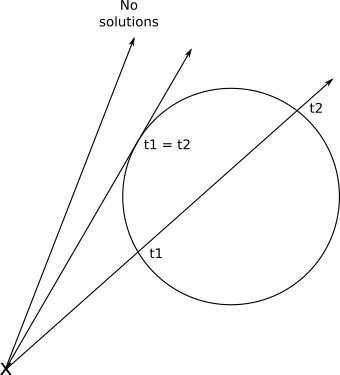
Fortunately, this has a geometric meaning. As you may remember, a quadratic equation may have no solutions, have one double solution or two different solutions, depending on the value of the discriminant$$${k_2}^2 -4k_1k_3$ .This exactly corresponds to the cases when the ray does not intersect the sphere, the ray touches the sphere and the ray enters and leaves the sphere:



If we take the value t and insert it into the equation of the ray, we finally get the intersection point P corresponding to this value t.

Rendering our first areas

To summarize - for each pixel on the canvas, we can calculate the corresponding point in the viewport. Knowing the position of the camera, we can express the equation of the beam that comes from the camera and passes through a given point of the viewing window. Having a sphere, we can calculate the point at which the ray intersects this sphere.

That is, we only need to calculate the intersection of the beam and each sphere, save the points closest to the camera and paint over the pixel on the canvas with the corresponding color. We are almost ready to render our first areas!

However, special attention should be paid to the parameter t. Returning to the beam equation:

$$

$$P = O + t(V - O)$$

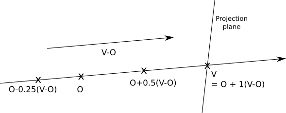
Since the initial point and the direction of the ray are constant, changing t in the set of real numbers, we get every point P on this ray. Notice that when$$t = 0 we get$t = 0$$$P = O , and$P = O$$$t = 1 we get$t = 1$$$$P = V$ .With negative numbers we get points in the opposite direction, that is, behind the camera . That is, we can divide the parameter area into three parts:

$$$t < 0$	Behind the camera
$$$0 \le t \le 1$	Between the camera and the projection plane
$$$t > 1$	Scene

Here is a diagram of the parameter area:


Notice that nothing in the intersection equation says that the sphere should be in front of the camera; the equation gives no solution at all for intersections behind the camera. Obviously, we do not need this; so we need to ignore all decisions when$$$t < 0$ . To avoid additional mathematical difficulties, we will limit the solutions. $$t > 1 , that is, we will render everything that isbehindthe projection plane.On the other hand, we do not need to set the upper limit of the value of t; we want to see objects in front of the camera, no matter how far they are. Since at later stages wewilllimit the length of the beam, we still need to add this formality and limit t to the upper value$t > 1$

$$+ ∞ (Note: in languages ​​in which infinity cannot be directly specified, a very large number will suffice.)Now we can formalize everything that was done in pseudo-code. In general, I will assume that the code has access to any data it needs, so we will not explicitly pass parameters, except for the most necessary ones. The main method now looks like this:$+\infty$

 O = <0, 0, 0>
for x in [-Cw / 2, Cw / 2] {
    for y in [-Ch / 2, Ch / 2] {
        D = CanvasToViewport (x, y)
        color = TraceRay (O, D, 1, inf)
        canvas.PutPixel (x, y, color)
     }
 } 

The function is CanvasToViewportvery simple:

 CanvasToViewport (x, y) {
    return (x * vw / cw, y * vh / ch, d)
 } 

In this code snippet d, this is the distance to the projection plane.

The method TraceRaycalculates the intersection of the ray with each sphere, and returns the color of the sphere at the nearest intersection point, which is in the required interval t:

 TraceRay (O, D, t_min, t_max) {
    closest_t = inf
    closest_sphere = NULL
    for sphere in scene.Spheres {
        t1, t2 = IntersectRaySphere (O, D, sphere)
        if t1 in [t_min, t_max] and t1 <closest_t
            closest_t = t1
            closest_sphere = sphere
        if t2 in [t_min, t_max] and t2 <closest_t
            closest_t = t2
            closest_sphere = sphere
     }
    if closest_sphere == NULL
        return BACKGROUND_COLOR
    return closest_sphere.color
 } 

Oin this code snippet, this is the starting point of the beam; Although we emit rays from a camera that is located at the origin point, at later stages it may be located elsewhere, so this value should be a parameter. The same applies to t_minand t_max.

Note that when the beam does not intersect the sphere, it must still return some color — in most of the examples I chose white for this.

And finally, IntersectRaySpherejust solves the quadratic equation:

 IntersectRaySphere (O, D, sphere) {
    C = sphere.center
    r = sphere.radius
    oc = O - C

    k1 = dot (D, D)
    k2 = 2 * dot (OC, D)
    k3 = dot (OC, OC) - r * r

    discriminant = k2 * k2 - 4 * k1 * k3
    if discriminant <0:
        return inf, inf

    t1 = (-k2 + sqrt (discriminant)) / (2 * k1)
    t2 = (-k2 - sqrt (discriminant)) / (2 * k1)
    return t1, t2
 } 

Let's set a very simple scene:



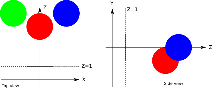
In the pseudo language of the scene, it will be set like this:

 viewport_size = 1 x 1
projection_plane_d = 1
sphere {
    center = (0, -1, 3)
    radius = 1
    color = (255, 0, 0) # Red
 }
sphere {
    center = (2, 0, 4)
    radius = 1
    color = (0, 0, 255) #Blue
 }
sphere {
    center = (-2, 0, 4)
    radius = 1
    color = (0, 255, 0) # Green
 } 

Then if we run the algorithm for this scene, then we will finally be rewarded with the look of an incredible scene obtained by ray tracing:



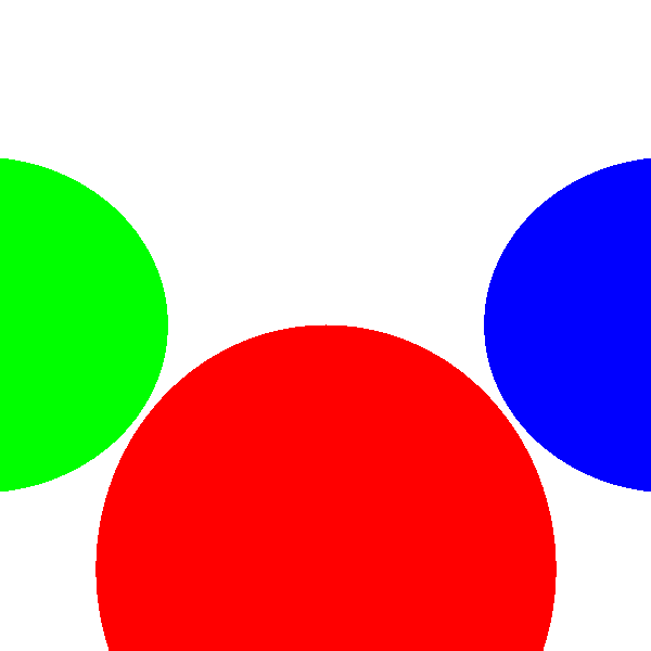
Source code and working demo >>

I know this is a bit disappointing. Where are the reflections, the shadows and the beautiful appearance? We all get it, because we have just started. But this is a good start - the spheres look like circles, and this is better than if they looked like cats. They do not look like spheres because we have missed an important component that allows a person to determine the shape of an object - how it interacts with the light.

Lighting

The first step to add “realism” to our scene rendering will be a lighting simulation. Lighting is an incredibly complex topic, so I’ll present a very simplified model, sufficient for our purposes. Some parts of this model are not even close to the physical models, they are just quick and good looking.

We will start with some simplifying assumptions that make life easier for us.

First, we will declare that all lighting is white. This will allow us to characterize any light source with a single real number i, called the brightness of the light. The simulation of color lighting is not so complicated (only three brightness values ​​are needed, one per channel, and the calculation of all colors and lighting per channel), but to make our work easier, I will not do it.

Secondly, we will get rid of the atmosphere. This means that the lighting does not become less bright, regardless of their range. The attenuation of the brightness of light depending on the distance is also not too difficult to implement, but for clarity, we will skip it for now.

Light sources

Light must come from somewhere . In this section, we will define three different types of light sources.

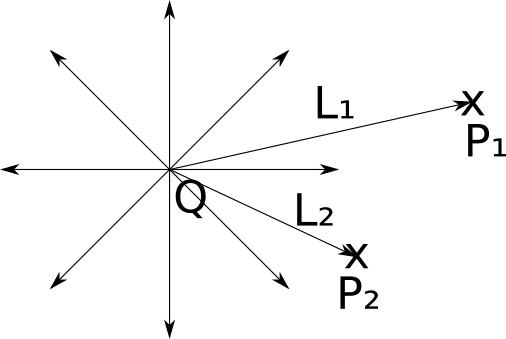
Point sources

A point source emits light from a fixed point in space, called its position . Light is emitted evenly in all directions; this is why it is also called omnidirectional lighting . Therefore, a point source is completely characterized by its position and brightness.

Incandescent bulbs are a good example from the real world, the approximation of which is a point source of illumination. Although the incandescent lamp does not emit light from one point and it is not completely omnidirectional, but the approximation is quite good.

Let's set the vector$$→ L as the direction from point P in the scene to the light source Q. This vector, called thelight vector, is simply equal to$\vec{L}$$$$Q - P$ . Note that since Q is fixed and P can be any point on the scene, in general $$→ L will be different for each point of the scene.$\vec{L}$

Directed Sources

If a point source is a good approximation of an incandescent lamp, then what can serve as an approximation of the sun?

This is a tricky question, and the answer depends on what you want to render.

On the scale of the Solar System, the Sun can be approximately considered as a point source. In the end, it emits light from a point (albeit a fairly large one) and emits it in all directions, that is, it fits both requirements.

However, if in your scene the action takes place on Earth, then this is not a very good approximation. The sun is so far away that each ray of light will actually have the same direction (Note: this approximation remains on a city scale, but not at longer distances - in fact. The ancient Greeks were able to calculate the radius of the Earth with surprising accuracy from different directions sunlight in various places.). Although it can be approximated using a point source far from the scene, this distance and the distance between objects in the scene are so different in magnitude that errors in the accuracy of numbers may appear.

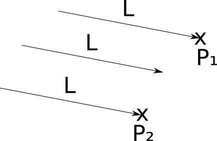
For such cases, we will set the directional light sources.. Like point sources, a directional source has brightness, but unlike them, it has no position. Instead, he has a direction . You can perceive it as an infinitely distant point source, shining in a certain direction.

In the case of point sources, we need to compute a new light vector.$$→ L for each point P of the scene, but in this case$\vec{L}$$$→ L is set. In a scene with the sun and the earth$\vec{L}$$$$\vec{L}$ will be equal to $$$(\text{ }) - (\text{ })$ .

Ambient lighting

Is it possible to model any real-world illumination as a point or directional source? Almost always yes (Note: but this will not necessarily be simple; zonal illumination (imagine the source behind the diffuser) can be approximated by a multitude of point sources on its surface, but it is difficult, more expensive to calculate, and the results are not ideal.). Are these two types of sources sufficient for our purposes? Unfortunately not.

Imagine what is happening on the moon. The only significant source of lighting nearby is the sun. That is, the "front half" of the Moon relative to the Sun receives all the lighting, and the "back half" is in complete darkness. We see it from different angles on Earth, and this effect creates what we call the "phases" of the Moon.

However, the situation on Earth is slightly different. Even the points that do not receive lighting directly from the light source are not completely in the dark (just look at the floor under the table). How do the rays of light reach these points if the “view” of the sources of illumination is somehow blocked?

As I mentioned in the section Color Modelswhen light falls on an object, part of it is absorbed, but the rest is scattered in the scene. This means that the light can come not only from sources of illumination, but also from other objects that receive it from sources of illumination and scatter it back. But why stop there? The diffuse illumination in turn falls on some other object, a part of it is absorbed, and a part is again scattered in the scene. With each reflection, the light loses some of its brightness, but theoretically you can continue ad infinitum (Note: in fact, no, because the light has a quantum nature, but close enough to this.).

This means that every object should be considered a source of lighting.. As you can imagine, this greatly increases the complexity of our model, so we will not go this way (Note: but you can at least google Global Illumination and look at the beautiful images.).

But we still do not want every object to be either illuminated directly, or completely dark (unless we render the model of the solar system). To overcome this barrier, we will define a third type of light source, called ambient light , which is characterized only by brightness. It is believed that it is the unconditional contribution of lighting to each point of the scene. This is a very powerful simplification of the extremely complex interaction between light sources and scene surfaces, but it works.

Illumination of one point

In general, there will be one ambient light source in the scene (because ambient light has only a brightness value, and any number of them will trivially combine into a single ambient light source) and an arbitrary number of point and directional sources.

To calculate the illumination of a point, we just need to calculate the amount of light contributed by each source and add them up to get one number representing the total amount received by the illumination point. Then we can multiply the color of the surface at this point by this number to get a properly lit color.

So, what happens when a ray of light with a direction$$→ L from a directional or point source falls on a point P of some object in our scene? Intuitively, we can break objects into two general classes, depending on how they behave with light: "matte" and "shiny." Since most of the objects around us can be considered "dull", then we will begin with them.$\vec{L}$

Diffuse scattering

When a beam of light falls on a matte object, because of the irregularity of its surface at the microscopic level, it reflects the beam into the scene evenly in all directions, that is, a “diffuse” (“diffuse”) reflection is obtained.

To see this, carefully look at some matte object, for example, a wall: if you move along the wall, its color does not change. That is, the light you see, reflected from the object, is the same regardless of where you are looking at the object.

On the other hand, the amount of reflected light depends on the angle between the light beam and the surface. Intuitively, this is understandable - the energy transferred by the beam, depending on the angle, should be distributed over a smaller or larger surface, that is, the energy per unit area reflected in the scene will be higher or lower, respectively:



To express it mathematically, let's characterize the orientation of the surface along its normal vector . The normal vector, or simply "normal" is a vector perpendicular to the surface at some point. It is also a unit vector, that is, its length is 1. We will call this vector$$$\vec{N}$ .

Diffuse reflection simulation

So, a ray of light with direction $$→ L and brightness$\vec{L}$$$I falls on the surface with normal$I$$$$\vec{N}$ . What part $$I is reflected back to the scene as a function of$I$$$$I$ , $$$\vec{N}$ and $$$\vec{L}$ ?

For a geometric analogy, let us imagine the brightness of the light as the “width” of the beam. Its energy is distributed over the surface size$$$A$ . When $$$\vec{N}$ and $$→ L have one direction, that is, the beam is perpendicular to the surface,$\vec{L}$$$I = A , which means that the energy reflected per unit area is equal to the incident energy per unit area;$I = A$ < $$${I \over A} = 1$ . On the other hand, when the angle between $$$\vec{L}$ and $$→ N approaches$\vec{N}$$$$90^\circ$ , $$A approaches$A$$$∞ , that is, the energy per unit area approaches 0;$\infty$$$$\lim_{A \to \infty} {I \over A} = 0$ .But what happens in between?

The situation is shown in the diagram below. We know$$$\vec{N}$ , $$$\vec{L}$ and $$$P$ ; I added corners $$$\ alpha$ and $$β as well as points$\beta$$$$Q$ , $$$\vec{R}$ and $$S to make related entries easier. Since technically the beam of light does not have a width, so we will assume that everything happens on an infinitely small flat portion of the surface. Even if it is the surface of a sphere, the area under consideration is so infinitely small that it is almost flat relative to the size of the sphere, just as the Earth looks flat at small scales. Beam of light with a width$S$





$$I falls to the surface at point$I$$$P at an angle$P$$$$\beta$ . Normal at $$$P$ equals $$→ N , and the energy transferred by the beam is distributed over$\vec{N}$$$$A$ . We need to calculate $$${I \over A}$ .

We assume $$S R "width" of the beam. By definition, it is perpendicular$SR$$$→ L , which is also the direction$\vec{L}$$$$PQ$ . therefore $$$PQ$ and $$Q R form a right angle, turning$QR$$$P Q R in a right triangle. One of the corners$PQR$

$$$PQR$ equals $$90 ∘ , and the other -$90^\circ$$$$\beta$ . Then the third angle is $$$90^\circ - \beta$ . But it should be noted that $$$\vec{N}$ and $$P R also form a right angle, i.e.$PR$$$α + β must also be$\alpha + \beta$$$$90^\circ$ . Consequently, $$$\widehat{QRP} = \alpha$ :



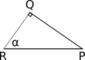
Let's look at the triangle $$$PQR$ . Its angles are equal $$$\ alpha$ , $$$\beta$ and $$$90^\circ$ . Side $$$QR$ equals $$I2 , and the side$I \over 2$$$$PR$ equals $$$A \over 2$ .

And now ... trigonometry to the rescue! By definition$$$cos(\alpha) = {QR \over PR}$ ; replace $$$QR$ on $$$I \over 2$ , but $$$PR$ on $$A2 , and we get$A \over 2$

$$

$$cos(\alpha) = { {I \over 2} \over {A \over 2} }$$

which translates into

$$

$$cos(\alpha) = {I \over A}$$

We are almost done. $$ a l p h a is the angle between$\ alpha$$$$\vec{N}$ and $$→ L , that is$\vec{L}$$$c o s ( α ) can be expressed as$cos(\alpha)$

$$

$$cos(\alpha) = {{\langle \vec{N}, \vec{L} \rangle} \over {|\vec{N}||\vec{L}|}}$$

And finally

$$

$${I \over A} = {{\langle \vec{N}, \vec{L} \rangle} \over {|\vec{N}||\vec{L}|}}$$

So, we have obtained a very simple equation relating the reflected part of the world to the angle between the normal to the surface and the direction of the light.

Note that with more angles$$$90^\circ$ value $$c o s ( α ) becomes negative. If we do not hesitate to use this value, then as a result we get light sources thatsubtractlight. It has no physical meaning; angle more$cos(\alpha)$$$90 ∘ simply means that the light actually reaches theback of thesurface, and does not contribute to the illumination of the illuminated point. That is, if$90^\circ$$$c o s ( α ) becomes negative, then we consider it equal$cos(\alpha)$$$$0$ .

Diffuse reflection equation

Now we can formulate an equation to calculate the total amount of light produced by a point $$P with normal$P$$$→ N in a scene with ambient lighting brightness$\vec{N}$$$$I_A$ and $$n point or directional light sources with brightness$n$$$I n and light vectors$I_n$$$→ L n or known (for directional sources), or calculated for P (for point sources):$\vec{L_n}$

$$

$$I_P = I_A + \sum_{i = 1}^{n} I_i {{\langle \vec{N}, \vec{L_i} \rangle} \over {|\vec{N}||\vec{L_i}|}}$$

It is worth repeating again that the members in which $$⟨ → N , → L i ⟩ < 0 should not be added to the light point.$\langle \vec{N}, \vec{L_i} \rangle < 0$

Sphere normals

The only trifle is missing here: where do the normals come from?

This question is much more cunning than it seems, as we will see in the second part of the article. Fortunately, for the case we are considering there is a very simple solution: the normal vector of any point of the sphere lies on a straight line passing through the center of the sphere. That is, if the center of the sphere is$$C , then the direction of the normal point$C$$$$P$ equally $$$P - C$ :



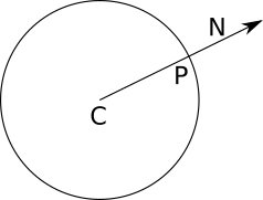
Why did I write “normal direction” instead of “normal”? In addition to perpendicularity to the surface, the normal should be a unit vector; it would be fair if the radius of the sphere were equal$$1 , which is not always true. To calculate the normal itself, we need to divide the vector by its length, thus obtaining the length$1$$$$1$ :

$$

$$\vec{N} = {{P - C} \over {|P - C|}}$$

This is mainly of theoretical interest, because the lighting equation written above contains a division by $$| → N | but a good approach would be to create "true" normals; This will simplify our work in the future.$|\vec{N}|$

Diffuse reflection rendering

Let's translate all this into pseudocode. First, let's add a couple of sources of lighting to the scene:

 light {
    type = ambient
    intensity = 0.2
 }
light {
    type = point
    intensity = 0.6
    position = (2, 1, 0)
 }
light {
    type = directional
    intensity = 0.2
    direction = (1, 4, 4)
 } 

Note that the brightness conveniently adds up to $$1.0 , because it follows from the lighting equation that no point can have a luminance higher than one. This means that we will not get areas with “too much exposure”. The lighting equation is quite simple to convert to pseudocode:$1.0$

 ComputeLighting (P, N) {
    i = 0.0
    for light in scene.Lights {
        if light.type == ambient {
            i + = light.intensity
         } else {
            if light.type == point
                L = light.position - P
             else
                L = light.direction

            n_dot_l = dot (N, L)
            if n_dot_l> 0
                i + = light.intensity * n_dot_l / (length (N) * length (L))
         }
     }
    return i
 } 

And the only thing left is to use ComputeLightingc TraceRay. We will replace the string that returns the color of the sphere.

 return closest_sphere.color 

to this fragment:

 P = O + closest_t * D # intersection calculation
    N = P - closest_sphere.center # calculating the sphere normal at the intersection point
    N = N / length (N)
    return closest_sphere.color * ComputeLighting (P, N) 

Just for fun, let's add a big yellow sphere:

 sphere {
    color = (255, 255, 0) # Yellow
    center = (0, -5001, 0)
    radius = 5000
 } 

We are launching the renderer, and see - the spheres have finally begun to look like spheres!



Source code and working demo >>

But wait, how did the big yellow sphere turn into a flat yellow floor?

It was not there, it’s just so big relative to the other three, and the camera is so close to it that it looks flat. Just as our planet looks flat when we stand on its surface.

Reflection from a smooth surface

Now we turn our attention to the "shiny" objects. Unlike "matte" objects, "shiny" change their appearance when you look at them from different angles.

Take a billiard ball or a car that has just been washed. In such objects, a special pattern of light propagation appears, usually with bright areas that seem to move when you walk around them. Unlike matte objects, how you perceive the surface of these objects actually depends on the point of view.

Notice that the red billiard balls remain red if you take a few steps back, but the bright white spot, giving them a “shiny” look, seems to move. This means that the new effect does not replace the diffuse reflection, but complements it.

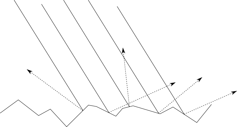
Why is this happening?We can start with why this does not happen on matte objects. As we saw in the previous section, when a beam of light falls on the surface of a frosted object, it is scattered evenly back into the scene in all directions. It is intuitively clear that this is due to the irregularity of the object's surface, that is, at the microscopic level, it resembles many small surfaces directed in random directions:



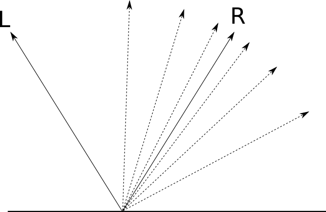
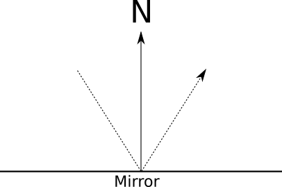
But what if the surface is not so uneven? Let's take the other extreme - a perfectly polished mirror. When a beam of light falls on a mirror, it is reflected in a single direction that is symmetrical to the angle of incidence relative to the normal of the mirror. If we call the direction of the reflected light$$→ R and agree that$\vec{R}$$$→ L indicatesalight source, we get the following situation:Depending on the degree of "polished" surface, it is more or less like a mirror; that is, we get a “mirror” reflection (specular reflection, from the Latin “speculum”, that is, a “mirror”). For a perfectly polished mirror incident beam$\vec{L}$





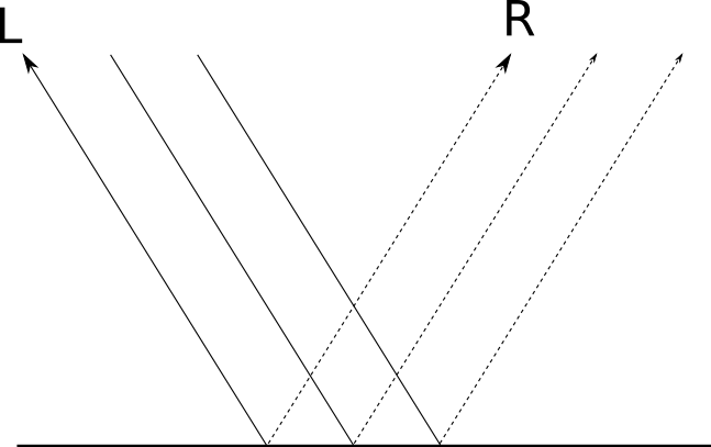
$$→ L is reflected in a single direction.$\vec{L}$$$$\vec{R}$ . This is what allows us to clearly see objects in the mirror: for each incident beam $$→ L is the only reflected ray.$\vec{L}$$$$\vec{R}$ .But not every object is perfectly polished; although most of the light is reflected in the direction$$→ R , part of it is reflected in directions close to$\vec{R}$$$$\vec{R}$ ; the closer to $$→ R , the more light is reflected in this direction. The “brilliance” of an object determines how quickly the reflected light decreases when away from$\vec{R}$$$$\vec{R}$ :



We are interested in how to find out how much light from $$→ L is reflected back in the direction of our point of view (because it is the light that we use to determine the color of each point).$\vec{L}$ If a $$→ V is the “view vector” indicating from$\vec{V}$$$P into the camera, and$P$$$ a l p h a - the angle between$\ alpha$$$$\vec{R}$ and $$→ V , this is what we have:$\vec{V}$



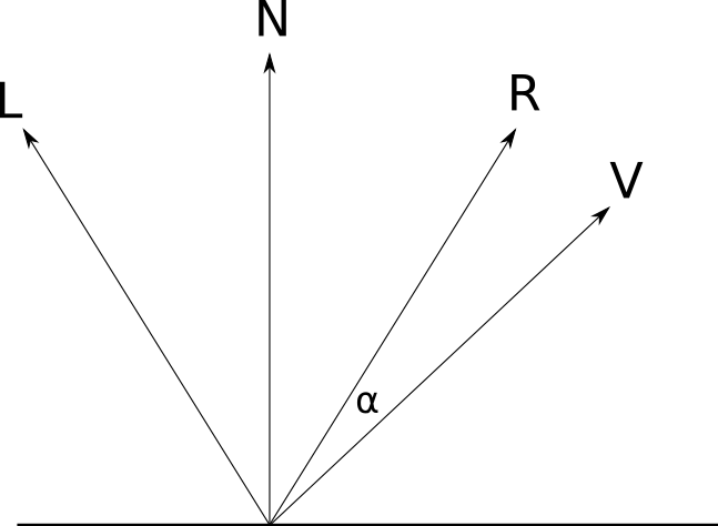
With $$α = 0 ∘ reflects the whole world.$\alpha = 0^\circ$ With $$α = 90 ∘ light is not reflected. As in the case of diffuse reflection, we need a mathematical expression to determine what happens at intermediate values.$\alpha = 90^\circ$$$$\ alpha$ .

Modeling "mirror" reflection

Remember how I mentioned earlier that not all models are based on physical models? Well, here is one example of this. The model presented below is arbitrary, but it is used, because it is easy to calculate and looks good.

Let's take$$$cos(\alpha)$ . He has good properties: $$$cos(0) = 1$ , $$c o s ( ± 90 ) = 0 , and the values ​​gradually decrease from$cos(\pm 90) = 0$$$$0$ before $$90 along a very beautiful curve:$90$



$$c o s ( α ) meets all the requirements for the “mirror” reflection function, so why not use it? But we lack one more detail. In this formulation, all objects shine the same. How to change the equation to obtain different degrees of brilliance? Remember that this gloss is a measure of how quickly the reflection function decreases with increasing$cos(\alpha)$



$$$\ alpha$ . A very simple way to get different light curves is to calculate the degree $$c o s ( α some positive indicator$cos(\alpha$$$$s$ . Insofar as $$0 ≤ c o s ( α ) ≤ 1 , it is obvious that$0 \le cos(\alpha) \le 1$$$$0 \le cos(\alpha)^s \le 1$ ; i.e $$c o s ( α ) s behaves exactly the same as$cos(\alpha)^s$$$c o s ( α , only “already”.$cos(\alpha$ Here is $$c o s ( α ) s for different values$cos(\alpha)^s$$$$s$ :



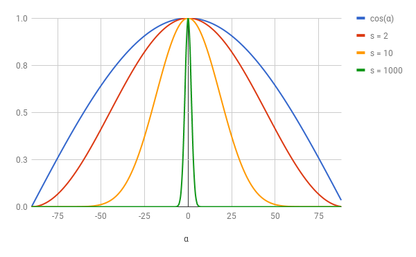
The larger the value $$s , the “already” becomes the function in the vicinity$s$$$0 , and the more brilliant the object looks.$0$

$$s is usually calledthe reflection index, and it is a surface property. Since the model is not based on physical reality, the values$s$$$s can only be determined by trial and error, that is, by adjusting the values ​​until they start to look “natural” (Note: for using a model based on physics, see the two-beam reflectance function (DFOS)). Let's unite everything together. Ray$s$

$$→ L falls to the surface at$\vec{L}$$$P , where the normal is$P$$$→ N , and the reflection index -$\vec{N}$$$$s$ . How much light is reflected in the direction of the view $$$\vec{V}$ ?

We have already decided that this value is $$$cos(\alpha)^s$ where $$ a l p h a is the angle between$\ alpha$$$$\vec{V}$ and $$→ R , which in turn is$\vec{R}$$$→ L , reflected relatively$\vec{L}$$$$\vec{N}$ . That is, the first step is to calculate $$$\vec{R}$ of $$$\vec{N}$ and $$$\vec{L}$ .

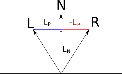
We can decompose $$→ L into two vectors$\vec{L}$$$$\vec{L_P}$ and $$→ L N such that$\vec{L_N}$$$$\vec{L} = \vec{L_P} + \vec{L_N}$ where $$→ L N is parallel$\vec{L_N}$$$$\vec{N}$ , but $$→ L P is perpendicular$\vec{L_P}$$$$\vec{N}$ :



$$→ L N is a projection.$\vec{L_N}$$$$\vec{L}$ on $$$\vec{N}$ ; on the properties of the scalar product and based on the fact that $$| → N | = 1 , the length of this projection is equal to$|\vec{N}| = 1$$$$\langle \vec{N}, \vec{L} \rangle$ . We have determined that $$→ L N will be parallel$\vec{L_N}$$$→ N , therefore$\vec{N}$$$$\vec{L_N} = \vec{N} \langle \vec{N}, \vec{L} \rangle$ .

Insofar as $$→ L = → L P + → L N , we can immediately get$\vec{L} = \vec{L_P} + \vec{L_N}$$$$\vec{L_P} = \vec{L} - \vec{L_N} = \vec{L} - \vec{N} \langle \vec{N}, \vec{L} \rangle$ .

Now look at $$$\vec{R}$ ; because it is symmetrical $$→ L relative$\vec{L}$$$→ N , its component, parallel$\vec{N}$$$→ N , same as u$\vec{N}$$$→ L , and the perpendicular component is opposite to the component$\vec{L}$$$$\vec{L}$ ; i.e $$$\vec{R} = \vec{L_N} - \vec{L_P}$ :



Substituting the expressions obtained earlier, we get

$$

$$\vec{R} = \vec{N} \langle \vec{N}, \vec{L} \rangle - \vec{L} + \vec{N} \langle \vec{N}, \vec{L} \rangle$$

and simplifying a little, we get

$$

$$\vec{R} = 2\vec{N} \langle \vec{N}, \vec{L} \rangle - \vec{L}$$

The value of the "mirror" reflection

Now we are ready to write the equation of “mirror” reflection:

$$

$$\vec{R} = 2\vec{N} \langle \vec{N}, \vec{L} \rangle - \vec{L}$$

$$

$$I_S = I_L \left( {{\langle \vec{R}, \vec{V} \rangle} \over {|\vec{R}||\vec{V}|}} \right)^s$$

As with diffuse lighting, $$c o s ( α ) can be negative, and again we should ignore it. In addition, not every object should be brilliant; for such objects (which we will present through$cos(\alpha)$$$s = - 1 ) the value of “specularity” will not be calculated at all.$s = -1$

Rendering with "mirror" reflections

Let's add to the scene the “mirror” reflections we were working on. First, we make some changes to the scene itself:

 sphere {
    center = (0, -1, 3)
    radius = 1
    color = (255, 0, 0) # Red
    specular = 500 # Brilliant
 }
sphere {
    center = (-2, 1, 3)
    radius = 1
    color = (0, 0, 255) #Blue
    specular = 500 # Brilliant
 }
sphere {
    center = (2, 1, 3)
    radius = 1
    color = (0, 255, 0) # Green
    specular = 10 # A bit shiny
 }
sphere {
    color = (255, 255, 0) # Yellow
    center = (0, -5001, 0)
    radius = 5000
    specular = 1000 # Very brilliant
 } 

In the code, we need to change ComputeLightingit to calculate the “specularity” value if necessary and add it to the general lighting. Notice that he now needs$$$\vec{V}$ and $$$s$ :

 ComputeLighting (P, N, V, s) {
    i = 0.0
    for light in scene.Lights {
        if light.type == ambient {
            i + = light.intensity
         } else {
            if light.type == point
                L = light.position - P
             else
                L = light.direction

            # Diffusion
            n_dot_l = dot (N, L)
            if n_dot_l> 0
                i + = light.intensity * n_dot_l / (length (N) * length (L))

            # Mirror
            if s! = -1 {
                R = 2 * N * dot (N, L) - L
                r_dot_v = dot (R, V)
                if r_dot_v> 0
                    i + = light.intensity * pow (r_dot_v / (length (R) * length (V)), s)
             }
         }
     }
    return i
 } 

Finally, we need to change TraceRayit to pass on new parameters ComputeLighting.$$s is obvious; It is taken from the data sphere. But what about$s$$$$\vec{V}$ ? $$→ V is the vector pointing from the object to the camera. Fortunately, inwe already have a vector directed from the camera to the object - this$\vec{V}$TraceRay$$→ D , the direction of the traced beam!$\vec{D}$ I.e $$→ V is just$\vec{V}$$$$-\vec{D}$ .

Here is the new code TraceRaywith a “mirror” reflection:

 TraceRay (O, D, t_min, t_max) {
    closest_t = inf
    closest_sphere = NULL
    for sphere in scene.Spheres {
        t1, t2 = IntersectRaySphere (O, D, sphere)
        if t1 in [t_min, t_max] and t1 <closest_t
            closest_t = t1
            closest_sphere = sphere
        if t2 in [t_min, t_max] and t2 <closest_t
            closest_t = t2
            closest_sphere = sphere
     }
    if closest_sphere == NULL
        return BACKGROUND_COLOR

    P = O + closest_t * D # Calculate intersection
    N = P - closest_sphere.center # Calculate the sphere normal at the intersection point
    N = N / length (N)
    return closest_sphere.color * ComputeLighting (P, N, -D, sphere.specular)
 } 

And here is our reward for all this juggling with vectors:



Source code and working demo >>

Shadows

Where there is light and objects, there must be shadows. So where are our shadows?

Let's start with a more fundamental question. Why should there be shadows? Shadows appear where there is light, but its rays cannot reach the object, because there is another object in their path.

You will notice that in the previous section we were interested in angles and vectors, but we considered only the light source and the point that we need to paint, and completely ignored everything else that happens in the scene — for example, an object in the way.

Instead, we need to add a bit of logic, saying " if there is an object between a point and a source, then there is no need to add lighting coming from this source ."

We want to highlight the following two cases:



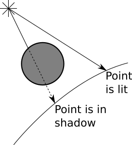
It seems that we have all the necessary tools for this.

Let's start with a directional source. We know$$$P$ ;This is the point that interests us. We know$$$\vec{L}$ ;This is part of the definition of the light source. Having$$$P$ and $$→ L , we can define a ray, namely$\vec{L}$$$P + t → L , which passes from a point to an infinitely distant light source. Does this beam intersect another object? If not, then there is nothing between the point and the source, that is, we can calculate the illumination from this source and add it to the total illumination. If it crosses, then we ignore this source. We already know how to calculate the nearest intersection between a ray and a sphere; we use it to trace the rays from the camera. We can again use it to calculate the nearest intersection between the ray of light and the rest of the scene. However, the parameters are slightly different. Instead of starting from the camera, the rays are emitted from$P + t\vec{L}$



$$$P$ . Direction is not equal $$$(V - O)$ , but $$$\vec{L}$ . And we are interested in intersections with everything after $$P for infinite distance; it means that$P$$$$t_{min} = 0$ and $$$t_{max} = +\infty$ .



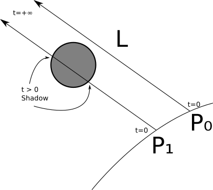
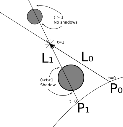
We can handle point sources in a very similar way, but with two exceptions. First, it is not set$$→ L , but it is very easy to calculate it from the position of the source and$\vec{L}$$$$P$ . Secondly, we are interested in any intersections, starting with $$P , but only until$P$$$L (otherwise, objectsbehind thelight source might create shadows!); that is, in this case$L$$$$t_{min} = 0$ and $$$t_{max} = 1$ .



There is one borderline case that we need to consider. Take a ray$$$P + t\vec{L}$ . If we search for intersections starting from $$t m i n = 0 , then we will most likely find the very$t_{min} = 0$$$$P$ at $$t = 0 because$t = 0$$$P really is on the sphere, and$P$$$$P + 0\vec{L} = P$ ;in other words, each object will cast shadows on itself (Note: more precisely, we want to avoid a situation in which a point, rather than the whole object, casts a shadow on itself; an object with a shape more complex than a sphere (namely, any concave an object can cast true shadows on itself!

The simplest way to handle this is to use the lower bound of values.$$$t$ instead $$0 small value$0$$$$\ epsilon$ . Geometrically, we want to make the beam start a little away from the surface, that is, next to $$P but not exactly in$P$$$$P$ . That is, for directional sources, the interval will be $$[ ϵ , + ∞ ] , and for point ones$[\epsilon, +\infty]$$$$[\epsilon, 1]$ .

Rendering with shadows

Let's turn this into pseudocode.

In the previous version, I TraceRaycalculated the nearest intersection of the ray-sphere, and then I calculated the lighting at the intersection. We need to extract the code of the nearest intersection, because we want to use it again to calculate the shadows:

 ClosestIntersection (O, D, t_min, t_max) {
    closest_t = inf
    closest_sphere = NULL
    for sphere in scene.Spheres {
        t1, t2 = IntersectRaySphere (O, D, sphere)
        if t1 in [t_min, t_max] and t1 <closest_t
            closest_t = t1
            closest_sphere = sphere
        if t2 in [t_min, t_max] and t2 <closest_t
            closest_t = t2
            closest_sphere = sphere
     }
    return closest_sphere, closest_t
 } 

The result TraceRayis much simpler:

 TraceRay (O, D, t_min, t_max) {
    closest_sphere, closest_t = ClosestIntersection (O, D, t_min, t_max)

    if closest_sphere == NULL
        return BACKGROUND_COLOR

    P = O + closest_t * D # Compute intersection
    N = P - closest_sphere.center # Compute sphere normal at intersection
    N = N / length (N)
    return closest_sphere.color * ComputeLighting (P, N, -D, sphere.specular)
 } 

Now we need to add ComputeLightinga shadow to the check:

 ComputeLighting (P, N, V, s) {
    i = 0.0
    for light in scene.Lights {
        if light.type == ambient {
            i + = light.intensity
         } else {
            if light.type == point {
                L = light.position - P
                t_max = 1
             } else {
                L = light.direction
                t_max = inf
             }

            # Shadow checking
            shadow_sphere, shadow_t = ClosestIntersection (P, L, 0.001, t_max)
            if shadow_sphere! = NULL
                 continue

            # Diffusion
            n_dot_l = dot (N, L)
            if n_dot_l> 0
                i + = light.intensity * n_dot_l / (length (N) * length (L))

            # Mirror
            if s! = -1 {
                R = 2 * N * dot (N, L) - L
                r_dot_v = dot (R, V)
                if r_dot_v> 0
                    i + = light.intensity * pow (r_dot_v / (length (R) * length (V)), s)
             }
         }
     }
    return i
 } 

Here’s what our newly rendered scene will look like:


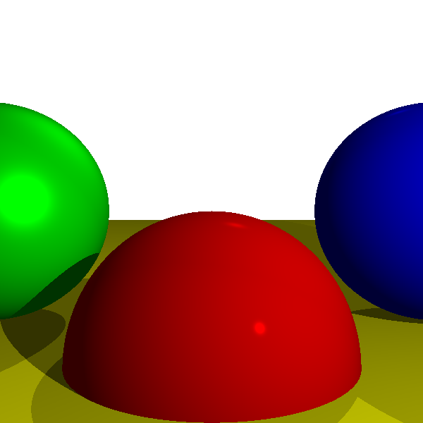
Source code and working demo >>

Now we are already doing something.

Reflection

We got shiny objects. But is it possible to create objects that actually behave like mirrors? Of course, in fact, their implementation in the ray tracer is very simple, but at first it may seem confusing.

Let's see how the mirrors work. When we look in the mirror, we see the rays of light reflected from the mirror. Rays of light are reflected symmetrically with respect to the surface normal:



Suppose we trace the beam and the closest intersection is a mirror. What color has a ray of light? Obviously, it is not the color of the mirror, but any color that has a reflected beam. All we need is to calculate the direction of the reflected beam and find out what was the color of the light falling from this direction. If only we had a function that returns for the given beam the color of the light falling from this direction ...

Oh, wait, we have it: it is called TraceRay.

So, we start with the main loop TraceRayto see what the beam emitted from the camera "sees". If it TraceRaydetermines that the ray sees a reflecting object, then it simply has to calculate the direction of the reflected ray and call ... itself.

At this stage, I suggest you re-read the last three paragraphs until you understand them. If this is your first time reading about recursive ray tracing, then you may need to reread a couple of times and think a bit before you really understand .

Take your time, I'll wait.

...

Now that the euphoria of this beautiful moment is eureka! Slept a little, let's formalize it a little.

The most important in all recursive algorithms is to prevent an infinite loop. In this algorithm, there is an obvious exit condition: when the beam either falls on a non-reflecting object, or when it does not fall on anything. But there is a simple case in which we can cater to an endless cycle: the effect of an endless corridor . It manifests itself when you put a mirror opposite another mirror and see endless copies of yourself in them!

There are many ways to prevent this problem. We will enter the recursion limit of the algorithm; he will control the "depth" to which he can go. Let's call him$$$r$ . With $$r = 0 , then we see objects, but without reflections.$r = 0$ With $$r = 1 we see some objects and reflections of some objects.$r = 1$ With $$r = 2 we see some objects, reflections of some objectsand reflections of some reflections of some objects.$r = 2$ And so on.In general, there is not much point in going deeper by more than 2-3 levels, because at this stage the difference is barely noticeable.

We will create another distinction. "Reflectability" should not matter "is or not" - objects can be partially reflective and partially colored. We will assign each surface a number from$$$0$ before $$1 , determining its reflectivity. Then we will mix the locally lit color and the reflected color in proportion to this number. Finally, you need to decide which parameters the recursive call should receive? The beam starts from the surface of the object, a point$1$

TraceRay$$$P$ . The direction of the beam is the direction of the light reflected from $$$P$ ;in TraceRaywe have$$→ D , that is, the direction from the camera to$\vec{D}$$$P , opposite to the movement of light, that is, the direction of the reflected beam will be$P$$$→ - D reflected on$\vec{-D}$$$$\vec{N}$ . Similar to what happens with shadows, we do not want objects to reflect themselves, so $$$t_{min} = \epsilon$ . We want to see objects reflected no matter how distant they are, therefore $$$t_{max} = +\infty$ . And the last - the recursion limit is one less than the recursion limit in which we are at the moment.

Rendering with reflection

Let's add reflection to the ray tracer code.

As before, first of all we change the scene:

 sphere {
    center = (0, -1, 3)
    radius = 1
    color = (255, 0, 0) # Red
    specular = 500 # Brilliant
    reflective = 0.2 # Slightly reflective
 }
sphere {
    center = (-2, 1, 3)
    radius = 1
    color = (0, 0, 255) #Blue
    specular = 500 # Brilliant
    reflective = 0.3 # A bit more reflective
 }
sphere {
    center = (2, 1, 3)
    radius = 1
    color = (0, 255, 0) # Green
    specular = 10 # A bit shiny
    reflective = 0.4 # Even more reflective
 }
sphere {
    color = (255, 255, 0) # Yellow
    center = (0, -5001, 0)
    radius = 5000
    specular = 1000 # Very brilliant
    reflective = 0.5 # half reflective
 } 

We use the “ray of reflection” formula in a couple of places, so we can get rid of it. She gets a ray$$→ R and normal$\vec{R}$$$→ N , returning$\vec{N}$$$→ R reflected on$\vec{R}$$$$\vec{N}$ :

 ReflectRay (R, N) {
    return 2 * N * dot (N, R) - R;
 } 

The only change in ComputeLightingis the replacement of the reflection equation to the challenge of this new one ReflectRay.

A small change has been made to the main method - we need to pass the TraceRayupper level limit of recursion:

 color = TraceRay (O, D, 1, inf, recursion_depth) 

A constant recursion_depthcan be given a reasonable value, for example, 3 or 5.

The only important changes occur near the end TraceRay, where we recursively calculate the reflections:

 TraceRay (O, D, t_min, t_max, depth) {
    closest_sphere, closest_t = ClosestIntersection(O, D, t_min, t_max)

    if closest_sphere == NULL
        return BACKGROUND_COLOR

    #   
    P = O + closest_t*D #   
    N = P - closest_sphere.center #       
    N = N / length(N)
    local_color = closest_sphere.color*ComputeLighting(P, N, -D, sphere.specular)

    #         ,   
    r = closest_sphere.reflective
    if depth <= 0 or r <= 0:
        return local_color

    #   
    R = ReflectRay(-D, N)
    reflected_color = TraceRay(P, R, 0.001, inf, depth - 1)

    return local_color*(1 - r) + reflected_color*r
 } 

Let the results speak for themselves:



Source code and working demo >>

To better understand the limit of the depth of recursion, let's take a closer look at the render with$$$r = 1$ :



But the same magnified view of the same scene, this time rendered with $$$r = 3$ :



As you can see, the difference is whether we see reflections of reflections of reflections of objects, or just reflections of objects.

Arbitrary camera

At the very beginning of the ray tracing discussion, we made two important assumptions: the camera is fixed in $$( 0 , 0 , 0 ) and sent to$(0, 0, 0)$$$→ Z + , and the direction “up” is$\vec{Z_+}$$$$\vec{Y_+}$ .In this section, we will get rid of these restrictions so that you can position the camera anywhere in the scene and direct it in any direction.

Let's start with position. You probably noticed that$$O is used throughout the pseudocode only once: as the starting point of the rays emanating from the camera in the top-level method. If we want to change the position of the camera. theonlything to do is use a different value for$O$$$$O$ .

Does the change in position affect the direction of the rays? Not at all. The direction of the rays is a vector passing from the camera to the projection plane. When we move the camera, the projection plane moves with the camera, that is, their relative positions do not change.

Let's now pay attention to the direction. Let's say we have a rotation matrix that rotates$$( 0 , 0 , 1 ) in the desired viewing direction, and$(0, 0, 1)$$$( 0 , 1 , 0 ) - in the right direction "up" (and since this is a rotation matrix, then by definition it should do what is required for$(0, 1, 0)$$$$(1, 0, 0)$ ). The position of the camera does not change if you simply rotate the camera around. But the direction changes, it just undergoes the same turn as the whole camera. That is, if we have a direction$$→ D and rotation matrix$\vec{D}$$$R , then rotated$R$$$D is just$D$$$$\vec{D}R$ .

Only the top level function changes:

 for x in [-Cw / 2, Cw / 2] {
    for y in [-Ch / 2, Ch / 2] {
        D = camera.rotation * CanvasToViewport (x, y)
        color = TraceRay (camera.position, D, 1, inf)
        canvas.PutPixel (x, y, color)
     }
 } 

This is how our scene looks when viewed from a different position and with a different orientation:



Source code and working demo >>

Where to go next

We will finish the first part of the work with a brief overview of some interesting topics that we did not explore.

Optimization

As stated in the introduction, we considered the most understandable way to explain and implement various possibilities. Therefore, the ray tracer is fully functional, but not very fast. Here are some ideas that you can explore on your own to speed up the work of the router. Just for fun, try to measure the execution time before and after their implementation. You will be very surprised!

Parallelization

The most obvious way to accelerate the work of the ray tracer is to trace several rays simultaneously. Since each beam emanating from the camera is independent of all the others, and most of the structures are read-only, we can trace one beam to each core of the central processor without much difficulty and difficulty due to synchronization problems.

In fact, ray tracers belong to a class of algorithms called extremely parallelizable precisely because their very nature makes it very easy to parallelize them.

Value caching

Consider the values ​​calculated IntersectRaySphereon which the ray tracer usually spends most of the time:

 k1 = dot (D, D)
    k2 = 2 * dot (OC, D)
    k3 = dot (OC, OC) - r * r 

Some of these values ​​are constant for the whole scene - as soon as you know how the spheres are located, r*rand dot(OC, OC)no longer change. You can calculate them once while loading the scene and store them in the spheres themselves; you just need to recount them if the spheres are to move in the next frame. dot(D, D)- this is a constant for a given beam, so you can calculate it in ClosestIntersectionand pass in IntersectRaySphere.

Shadow Optimization

If a point of an object is in the shadow relative to the light source, because another object is detected on the way, then there is a high probability that the neighboring point due to the same object is also in the shadow relative to the light source (this is called shadow consistency ):



That is When we search for objects between a point and a light source, we can first check whether the last object that shadows the previous point over the same light source imposes a shadow on the current point. If so, then we can finish; if not, then just continue to check the remaining objects in the usual way.

Similarly, when calculating the intersection between a ray of light and objects in the scene, in fact we do not need the nearest intersection - it is enough to know that there is at least one intersection. You can use a special version ClosestIntersectionthat returns the result as soon as it finds the first intersection (and for this we need to calculate and return not closest_tjust a boolean value).

Spatial structures

Calculating the intersection of the beam with each sphere is quite a big waste of resources. There are many data structures that allow you to drop entire groups of objects at one go without the need to calculate individual intersections.

A detailed examination of such structures does not relate to the subject of our article, but the general idea is this: suppose that we have several areas close to each other. You can calculate the center and radius of the smallest sphere containing all of these spheres. If the ray does not intersect this boundary sphere, then one can be sure that it does not intersect any sphere contained in it, and this can be done in one intersection check. Of course, if he crosses a sphere, then we still need to check if he crosses any of the spheres contained in it.

You can learn more about this by reading about the hierarchy of limiting volumes .

Subsampling

Here is an easy way to do a ray tracer in $$N times faster: calculate in$N$$$N times pixels smaller! Suppose we trace rays for pixels$N$

$$$(10, 100)$ and $$( 12 , 100 ) , and they fall on one object. You can logically assume that the ray is for a pixel.$(12, 100)$$$( 11 , 100 ) will also fall on the same object, skip the initial search for intersections with the entire scene and go directly to the color calculation at this point. If you do this in the horizontal and vertical directions, then you can perform a maximum of 75% less primary beam-scene cross-sectional calculations. Of course, one can easily miss a very thin object: unlike the ones considered earlier, this is the “wrong” optimization, because the results of its use are notidenticalto what we would get without it; in a sense, we are “cheating” on this economy. The trick is to figure out how to save properly, ensuring satisfactory results.$(11, 100)$

Other primitives

In the previous sections, we used spheres as primitives because it is convenient to manipulate them from a mathematical point of view. But having achieved this, you can simply add other primitives.

Note that from the point of view TraceRay, any object may be suitable, as long as it needs to calculate only two values: the value$$t for the nearest intersection between the ray and the object, and the normal at the intersection point. Everything else in the ray tracer does not depend on the type of object. Triangles are a good choice. First you need to calculate the intersection between the ray and the plane containing the triangle, and if there is an intersection, then determine whether the point is inside the triangle.$t$

Constructive block geometry

There is a very interesting type of objects that is relatively simple to implement: a boolean operation between other objects. For example, the intersection of two spheres can create something similar to a lens, and when subtracting a small sphere from a larger sphere, you can get something resembling a Death Star.

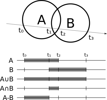
How it works?For each object, you can calculate the places where the ray enters and leaves the object; for example, in the case of a sphere, a ray enters$$m i n ( t 1 , t 2 ) and goes to$min(t_1, t_2)$$$$max(t_1, t_2)$ .Suppose we need to calculate the intersection of two spheres; the beam is inside the intersection when it is inside both spheres, and outside otherwise. In the case of subtraction, the beam is inside when it is inside the first object, but not inside the second.

More generally, if we want to calculate the intersection between a ray and$$$A \bigodot B$ (Where $$⨀ - any Boolean operator), then first you need to separately calculate the intersection of the ray$\bigodot$$$A and luch-$A$$$B , which gives us the "internal" interval of each object$B$$$$R_a$ and $$$R_b$ . Then we calculate $$R A ⨀ R B , which is in the "internal" interval$R_A \bigodot R_B$$$$A \bigodot B$ . We just need to find the first value. $$t , which is both in the "internal" interval and in the interval$t$$$[ t m i n , t m a x ] that interest us: Thenormal at the intersection point is either the normal of the object creating the intersection, or its opposite, depending on whether we look outside or inside the original object. Of course$[t_{min}, t_{max}]$





$$$A$ and $$B do not have to be primitive; they themselves can be the results of boolean operations! If we realize this purely, then we will not even need to knowwhatthey are, as long as we can get intersections and normals from them. Thus, we can take three spheres and calculate, for example,$B$$$$(A \cup B) \cap C$ .

Transparency

Not all objects must be opaque, some may be partially transparent.

The implementation of transparency is very similar to the implementation of reflection. When the beam falls on a partially transparent surface, we, as before, calculate the local and reflected color, but also calculate the additional color - the color of light passing through the object received by another call TraceRay. Then you need to mix this color with local and reflected colors, taking into account the transparency of the object, and that's it.

Refraction

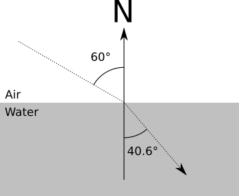
In real life, when a ray of light passes through a transparent object, it changes direction (therefore, when immersed in a straw in a glass of water, it looks “broken”). The change of direction depends on the refractive index of each material in accordance with the following equation:

$$

$${sin(\alpha_1) \over sin(\alpha_2)} = { n_2 \over n_1 }$$

Where $$$\ alpha_1$ and $$α 2 is the angle between the beam and the normal before and after crossing the surface, and$\alpha_2$$$$n_1$ and $$n 2 - the refractive indices of the material outside and inside objects.$n_2$

For example, $$n in about z d y x and approximately equal$n_{}$$$$1.0$ , but $$n in about d s approximately equal$n_{}$$$$1.33$ . That is, for a ray entering the water at an angle $$$60^\circ$ we get

$$

$${sin(60) \over sin(\alpha_2)} = {1.33 \over 1.0}$$

$$

$$sin(\alpha2) = {sin(60) \over 1.33}$$

$$

$$\alpha2 = arcsin({sin(60) \over 1.33}) = 40.628^\circ$$

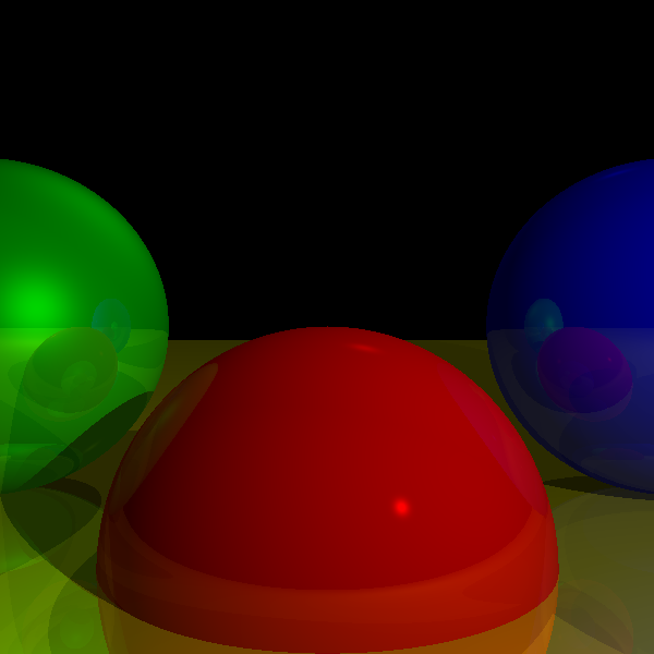
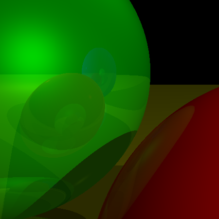
Stop for a moment and realize: if you implement a constructive block geometry and transparency, you can simulate a magnifying glass (the intersection of two spheres), which will behave like a physically correct magnifying glass!

Supersampling

Supersampling is the approximate opposite of subsampling, when we strive for accuracy instead of speed. Suppose that the rays corresponding to two neighboring pixels fall on two different objects. We need to color each pixel in the appropriate color.

However, do not forget about the analogy with which we started: each beam must specify the “determining” color of each square of the “grid” through which we look. Using one ray per pisle, we conditionally decide that the color of the ray of light passing through the middle of the square determines the whole square, but this may not be so.

This problem can be solved by tracing several rays per pixel - 4, 9, 16, and so on, and then averaging them to get the color of the pixel.

Of course, with this, the ray tracer becomes 4, 9 or 16 times slower, for the same reason that sub-sampling makes it in $$N times faster. Fortunately, there is a trade-off. We can assume that the properties of an object along its surface change smoothly, that is, the emission of 4 rays per pixel that fall on one object at slightly different points does not improve the look of the scene too much. Therefore, we can start from one ray per pixel and compare neighboring rays: if they fall on other objects or their color differs more than on a divided threshold value, then we apply a division of pixels to both.$N$

Ray tracer pseudocode

Below is the full version of the pseudo code we created in the ray tracing chapters:

 CanvasToViewport (x, y) {
    return (x * vw / cw, y * vh / ch, d)
 }


ReflectRay (R, N) {
    return 2 * N * dot (N, R) - R;
 }


ComputeLighting (P, N, V, s) {
    i = 0.0
    for light in scene.Lights {
        if light.type == ambient {
            i + = light.intensity
         } else {
            if light.type == point {
                L = light.position - P
                t_max = 1
             } else {
                L = light.direction
                t_max = inf
             }

            # Shadow checking
            shadow_sphere, shadow_t = ClosestIntersection (P, L, 0.001, t_max)
            if shadow_sphere! = NULL
                 continue

            # Diffusion
            n_dot_l = dot (N, L)
            if n_dot_l> 0
                i + = light.intensity * n_dot_l / (length (N) * length (L))

            # Glitter
            if s! = -1 {
                R = ReflectRay (L, N)
                r_dot_v = dot (R, V)
                if r_dot_v> 0
                    i + = light.intensity * pow (r_dot_v / (length (R) * length (V)), s)
             }
         }
     }
    return i
 }


ClosestIntersection (O, D, t_min, t_max) {
    closest_t = inf
    closest_sphere = NULL
    for sphere in scene.Spheres {
        t1, t2 = IntersectRaySphere (O, D, sphere)
        if t1 in [t_min, t_max] and t1 <closest_t
            closest_t = t1
            closest_sphere = sphere
        if t2 in [t_min, t_max] and t2 <closest_t
            closest_t = t2
            closest_sphere = sphere
     }
    return closest_sphere, closest_t
 }


TraceRay (O, D, t_min, t_max, depth) {
    closest_sphere, closest_t = ClosestIntersection (O, D, t_min, t_max)

    if closest_sphere == NULL
        return BACKGROUND_COLOR

    # Calculating local color
    P = O + closest_t * D # Calculating the intersection point
    N = P - closest_sphere.center # Calculate the sphere normal at the intersection point
    N = N / length (N)
    local_color = closest_sphere.color * ComputeLighting (P, N, -D, sphere.specular)

    # If we have reached the recursion limit or the object is not reflective, then we are done.
    r = closest_sphere.reflective
    if depth <= 0 or r <= 0:
        return local_color

    # Calculation of reflected color
    R = ReflectRay (-D, N)
    reflected_color = TraceRay (P, R, 0.001, inf, depth - 1)

    return local_color * (1 - r) + reflected_color * r
 }


for x in [-Cw / 2, Cw / 2] {
    for y in [-Ch / 2, Ch / 2] {
        D = camera.rotation * CanvasToViewport (x, y)
        color = TraceRay (camera.position, D, 1, inf)
        canvas.PutPixel (x, y, color)
     }
 } 

Here is the scene used to render the examples:

 viewport_size = 1 x 1
projection_plane_d = 1

sphere {
    center = (0, -1, 3)
    radius = 1
    color = (255, 0, 0) # Red
    specular = 500 # Brilliant
    reflective = 0.2 # Slightly reflective
 }
sphere {
    center = (-2, 1, 3)
    radius = 1
    color = (0, 0, 255) #Blue
    specular = 500 # Brilliant
    reflective = 0.3 # A bit more reflective
 }
sphere {
    center = (2, 1, 3)
    radius = 1
    color = (0, 255, 0) # Green
    specular = 10 # A bit shiny
    reflective = 0.4 # Even more reflective
 }
sphere {
    color = (255, 255, 0) # Yellow
    center = (0, -5001, 0)
    radius = 5000
    specular = 1000 # Very brilliant
    reflective = 0.5 # half reflective
 }


light {
    type = ambient
    intensity = 0.2
 }
light {
    type = point
    intensity = 0.6
    position = (2, 1, 0)
 }
light {
    type = directional
    intensity = 0.2
    direction = (1, 4, 4)
 }