Colorize a black and white photo using a neural network of 100 lines of code
Translation of the article Colorizing B & W Photos with Neural Networks .
Not so long ago, using neural networks, Amir Avni used a reddit / r / Colorization branch on Reddit , where people gather who are fond of hand-painted historical black-and-white images in Photoshop. All were amazed at the quality of the neural network. What takes up to a month of manual work can be done in a few seconds.
Let's reproduce and document the image processing process of Amir. First, look at some of the achievements and failures (at the bottom - the latest version).

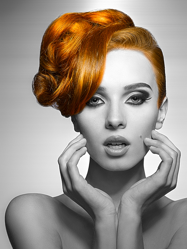
Original black and white photos taken from Unsplash .
')
Today, black and white photographs are usually painted by hand in Photoshop. Watch this video to get an idea of the enormous complexity of such work:
It can take a month to color a single image. We have to explore a lot of historical materials from that time. Up to 20 layers of pink, green and blue shadows are superimposed on the face alone to create the right shade.
This article is for beginners. If you are not familiar with the terminology of in-depth training of neural networks, then you can read the previous articles ( 1 , 2 ) and see the lecture by Andrey Karpaty.
In this article, you will learn how to build your own neural network for coloring images in three stages.
In the first part, we will deal with the basic logic. Let's build a frame of a neural network of 40 lines, this will be an “alpha” version of a coloring bot. This code is not very mysterious, it will help you to get acquainted with the syntax.
In the next step, we will make a generalizing (generalize) neural network - a “beta” version. She will already be able to color images that are not familiar to her.
In the "final" version, we will combine our neural network with a classifier. To do this, take Inception Resnet V2 , trained in 1.2 million images. A neural network will teach coloring on images with Unsplash .
If you can not wait, here is Jupyter Notebook with the alpha version of the bot. You can also look at the three versions on FloydHub and GitHub , and also the code used in all the experiments that were carried out on the FloydHub cloud video cards.
Basic logic
In this section, we will look at image rendering, talk about the theory of digital color and the basic logic of a neural network.
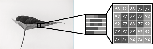
Black and white images can be represented as a grid of pixels. Each pixel has a brightness value in the range from 0 to 255, from black to white.
Color images consist of three layers: red, green and blue. Suppose you need to decompose in three channels a picture with a green leaf on a white background. You might think that the leaf will be presented only in the green layer. But, as you can see, it is in all three layers, because the layers determine not only color, but also brightness.
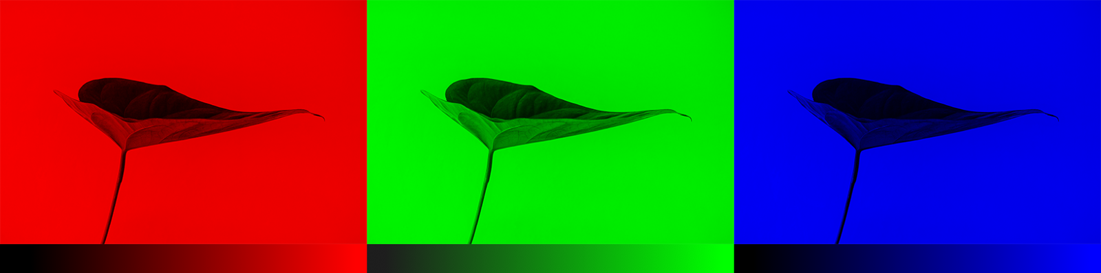
For example, to get white, we need to get an equal distribution of all colors. If you add the same amount of red and blue, then the green will become brighter. That is, in a color image using three layers color and contrast are encoded.

As in the black and white image, the pixels of each color image layer contain a value from 0 to 255. Zero means that this pixel in this layer does not have color. If there are zeros in all three channels, then the result is a black pixel in the picture.
As you know, the neural network establishes the relationship between input and output values. In our case, the neural network should find the connecting features between black and white and color images. That is, we are looking for properties by which we can compare the values from the black and white grid with the values from the three color ones.

f () is a neural network, [B & W] is input data, [R], [G], [B] is output data.
Alpha version
First, we will make a simple version of the neural network that will color the female face. As you add new features, you will become familiar with the basic syntax of our model.
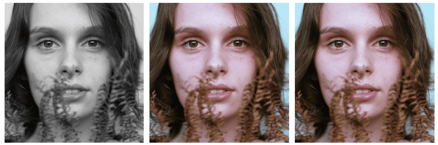
For 40 lines of code, we move from the left image - black and white - to the middle one, which is made by our neural network. The right picture is an original photograph, from which we made black and white. The neural network was trained and tested on one image, we will talk about this in the section on the beta version.
Color space
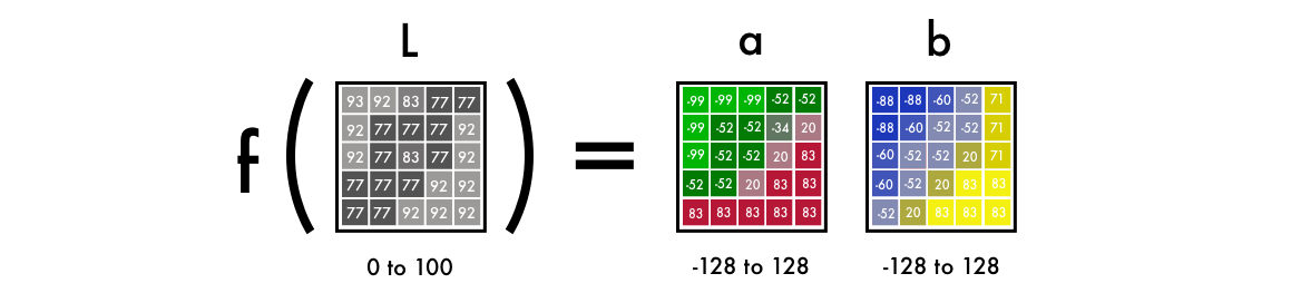
First, we use the algorithm for changing color channels from RGB to Lab. L means lightness, a and b are Cartesian coordinates that determine the position of a color in the range from green to red and from blue to yellow, respectively.
As you can see, the image in the Lab space contains one layer of grayscale, and three color layers are packed in two. Therefore, we can use the original black and white version in the final image. It remains to calculate two more channels.

Scientific fact: 94% of our eye retina receptors are responsible for determining the brightness. And only 6% of receptors recognize colors. Therefore, for you, a black and white image looks much clearer than color layers. This is another reason why we will use this image in the final version.
From grayscale to color
We take a layer with grayscale as input, and on its basis we will generate color layers a and b in the Lab color space. We will take it as the L-layer of the final picture.
To get two layers from one layer, we use convolutional filters. They can be represented as blue and red glass in 3D glasses. Filters determine what we see in the picture. They can emphasize or hide some part of the image so that our eye can extract the necessary information. A neural network can also create a new image using a filter or reduce several filters into one image.
In convolutional neural networks, each filter is automatically adjusted to make it easier to get the necessary output. We will add hundreds of filters and then put them together and get layers a and b.
Before proceeding to the details of the code, let's run it.
Deploying FloydHub Code
If you have not worked with FloydHub before, you can run the installation for now and watch the five-minute video tutorial or step-by-step instructions . FloydHub is the best and simplest way to deeply learn models on cloud-based video cards.
Alpha version
After installing FloydHub, enter the following command:
git clone https://github.com/emilwallner/Coloring-greyscale-images-in-KerasThen open the folder and initialize FloydHub.
cd Coloring-greyscale-images-in-Keras/floydhub
floyd init colornet
The FloydHub web panel will open in your browser. You will be prompted to create a new FloydHub project called colornet. When you create it, go back to the terminal and execute the same initialization command.
floyd init colornetRun the task:
floyd run --data emilwallner/datasets/colornet/2:data --mode jupyter --tensorboardA few explanations:
- With this command, we mounted a public dataset on FloydHub:
--dataemilwallner/datasets/colornet/2:data
On FloydHub you can view and use this and many other public datasets. - Enable Tensorboard with the command -
--tensorboard - Run the task in Jupyter Notebook mode using the command
--mode jupyter
If you can connect video cards to the task, add the
–gpu flag to the –gpu . Get about 50 times faster.Go to Jupyter Notebook. On the FloydHub website in the Jobs tab, click on the Jupyter Notebook link and locate the file:
floydhub/Alpha version/working_floyd_pink_light_full.ipynbOpen the file and on all cells press Shift + Enter.
Gradually increase the value of periods (epoch value) to understand how a neural network learns.
model.fit(x=X, y=Y, batch_size=1, epochs=1)Start with epochs = 1, then increase to 10, 100, 500, 1000 and 3000. This value shows how many times the network is trained in the image. As soon as you train the neural network, you will find the img_result.png file in the main folder.
# Get images
image = img_to_array(load_img('woman.png'))
image = np.array(image, dtype=float)

# Import map images into the lab colorspace
X = rgb2lab(1.0/255*image)[:,:,0]
Y = rgb2lab(1.0/255*image)[:,:,1:]
Y = Y / 128
X = X.reshape(1, 400, 400, 1)
Y = Y.reshape(1, 400, 400, 2)
model = Sequential()
model.add(InputLayer(input_shape=(None, None, 1)))

# Building the neural network
model = Sequential()
model.add(InputLayer(input_shape=(None, None, 1)))
model.add(Conv2D(8, (3, 3), activation='relu', padding='same', strides=2))
model.add(Conv2D(8, (3, 3), activation='relu', padding='same'))
model.add(Conv2D(16, (3, 3), activation='relu', padding='same'))
model.add(Conv2D(16, (3, 3), activation='relu', padding='same', strides=2))
model.add(Conv2D(32, (3, 3), activation='relu', padding='same'))
model.add(Conv2D(32, (3, 3), activation='relu', padding='same', strides=2))
model.add(UpSampling2D((2, 2)))
model.add(Conv2D(32, (3, 3), activation='relu', padding='same'))
model.add(UpSampling2D((2, 2)))
model.add(Conv2D(16, (3, 3), activation='relu', padding='same'))
model.add(UpSampling2D((2, 2)))
model.add(Conv2D(2, (3, 3), activation='tanh', padding='same'))

# Finish model
model.compile(optimizer='rmsprop',loss='mse')

#Train the neural network
model.fit(x=X, y=Y, batch_size=1, epochs=3000)
print(model.evaluate(X, Y, batch_size=1))

# Output colorizations
output = model.predict(X)
output = output * 128
canvas = np.zeros((400, 400, 3))
canvas[:,:,0] = X[0][:,:,0]
canvas[:,:,1:] = output[0]
imsave("img_result.png", lab2rgb(canvas))
imsave("img_gray_scale.png", rgb2gray(lab2rgb(canvas)))
FloydHub command to run this network:
floyd run --data emilwallner/datasets/colornet/2:data --mode jupyter --tensorboardTechnical explanation
Recall that at the entrance we have a grid representing a black and white image. And at the exit - two grids with color values. We created link filters between the input and output values. We have a convolutional neural network.
For training the network uses color images. We converted from RGB color space to Lab. The black and white layer is fed to the input, and two colored layers are obtained at the output.

We in one range compare (map) the calculated values with real, thereby comparing them with each other. The boundaries of the range from -1 to 1. To compare the calculated values, we use the activation function tanh (hyperbolic tangential). If you apply it to any value, the function returns a value in the range from -1 to 1.
Actual color values vary from —128 to 128. In Lab space, this is the default range. If each value is divided by 128, then all of them will be in the range from -1 to 1. Such a “normalization” allows us to compare the error of our calculation.
After calculating the resulting error, the neural network updates the filters to correct the result of the next iteration. The whole procedure is repeated cyclically until the error becomes minimal.
Let's understand the syntax of this code:
X = rgb2lab(1.0/255*image)[:,:,0]
Y = rgb2lab(1.0/255*image)[:,:,1:]
1.0 / 255 means we use a 24-bit RGB color space. That is, for each color channel we use values in the range from 0 to 255. This gives us 16.7 million colors.
But since the human eye can only recognize between 2 and 10 million colors, it does not make sense to use a wider color space.
Y = Y / 128Lab color space uses a different range. The color spectrum ab varies from —128 to 128. If we divide all the values of the output layer by 128, they will be within the range from -1 to 1, and then we can compare these values with those calculated by our neural network.
After using the
rgb2lab() function to convert the color space, we use the [:,:, 0] to select a black and white layer. This is the input to the neural network. [:,:, 1:] selects two color layers, red-green and blue-yellow.After learning the neural network, we perform the last calculation, which we translate into a picture.
output = model.predict(X)
output = output * 128
Here we feed a black and white image to the input and run it through a trained neural network. We take all the output values from -1 to 1 and multiply them by 128. So we get the correct colors in the Lab system.
canvas = np.zeros((400, 400, 3))
canvas[:,:,0] = X[0][:,:,0]
canvas[:,:,1:] = output[0]
Create a black RGB canvas by filling all three layers with zeros. Then copy the black and white layer from the test image and add two color layers. We turn the resulting array of pixel values into an image.
What have we learned while working on the alpha version
- Reading research is hard work . But it was enough to summarize the key points of the articles, and studying them became easier. It also helped to include some details in this article.
- You need to start small . Most of the implementations we found on the network consisted of 2–10 thousand lines of code. This makes it hard to get an idea of the basic logic. But if there is a simplified, basic version at hand, then it is easier to read and implement, and research.
- Do not be lazy to understand other people's projects . We had to look at a few dozen projects on coloring images on Github to determine the content of our code.
- Not everything works as planned . Perhaps, at first, your network will be able to create only red and yellow colors. For the first time, we used the Relu activation function for final activation. But it generates only positive values, and therefore the blue and green spectra are not available to it. This disadvantage was solved by adding the activation function tanh to convert the values along the Y axis.
- Understanding> speed . Many of the implementations we saw were executed quickly, but it was difficult to work with them. Therefore, we decided to optimize our code for the sake of adding new features, not execution.
Beta version
Offer the alpha versions to color the image in which she was not trained, and immediately understand what the main drawback of this version is. She can't handle it. The fact is that the neural network remembered the information. She did not learn to paint an unfamiliar image. And we will fix this in the beta version - we will teach the neural network to generalize.
Below is a beta version that colored test images.
Instead of using Imagenet, we created a public dataset with higher quality images on FloydHub . They are taken from Unsplash - a site where pictures of professional photographers are laid out. 9500 training images and 500 verification images.

Feature selector
Our neural network is looking for characteristics linking black and white images with their color versions.
Imagine that you need to color black and white pictures, but you can see only nine pixels on the screen at a time. You can view each picture from left to right and from top to bottom, trying to calculate the color of each pixel.

Let these nine pixels are on the edge of the woman's nostrils. As you understand, choosing the right color here is almost impossible, so you have to break the solution of the problem into stages.
First, we look for simple characteristic structures: diagonal lines, only black pixels, and so on. In each square of 9 pixels, we are looking for the same structure and delete everything that does not correspond to it. As a result, we created 64 new images from 64 of our minifilters.

Number of images processed by filters at each stage.
If we look through the images again, we will find the same small repeating structures that we have already identified. To better analyze the image, reduce its size by half.
Reduce the size in three stages.
We still have a 3x3 filter that needs to scan each image. But if we apply our simpler filters to new squares of nine pixels, we can find more complex structures. For example, a semicircle, a small dot or line. Again and again, we find the same repeating structure in the picture. This time we generate 128 new images processed by filters.
After a couple of steps, the processed images will look like this:

Again: you start by looking for simple properties, such as edges. As they are processed, the layers are combined into structures, then into more complex features, and in the end a face is obtained. Details are explained in this video:
The described process is very similar to computer vision algorithms. Here we use the so-called convolutional neural network, which combines several processed images to understand the contents of the entire image.
From extracting properties to color
The neural network operates on the principle of trial and error. First, it randomly assigns a color to each pixel. Then, for each pixel, it calculates errors and adjusts the filters so that in the next attempt to improve the results.
The neural network adjusts its filters based on the results with the largest error values. In our case, the neural network decides whether to color or not, and how to place different objects in the picture. First, she paints all objects in brown. This color is most similar to all other colors, so with it, using it produces the smallest errors.
Due to the monotony of the training data, the neural network tries to understand the differences between these or other objects. She still can not calculate more accurate color shades, we will deal with this when creating a full version of the neural network.
Here is the beta code:
# Get images
X = []
for filename in os.listdir('../Train/'):
X.append(img_to_array(load_img('../Train/'+filename)))
X = np.array(X, dtype=float)

# Set up training and test data
split = int(0.95*len(X))
Xtrain = X[:split]
Xtrain = 1.0/255*Xtrain

#Design the neural network
model = Sequential()
model.add(InputLayer(input_shape=(256, 256, 1)))
model.add(Conv2D(64, (3, 3), activation='relu', padding='same'))
model.add(Conv2D(64, (3, 3), activation='relu', padding='same', strides=2))
model.add(Conv2D(128, (3, 3), activation='relu', padding='same'))
model.add(Conv2D(128, (3, 3), activation='relu', padding='same', strides=2))
model.add(Conv2D(256, (3, 3), activation='relu', padding='same'))
model.add(Conv2D(256, (3, 3), activation='relu', padding='same', strides=2))
model.add(Conv2D(512, (3, 3), activation='relu', padding='same'))
model.add(Conv2D(256, (3, 3), activation='relu', padding='same'))
model.add(Conv2D(128, (3, 3), activation='relu', padding='same'))
model.add(UpSampling2D((2, 2)))
model.add(Conv2D(64, (3, 3), activation='relu', padding='same'))
model.add(UpSampling2D((2, 2)))
model.add(Conv2D(32, (3, 3), activation='relu', padding='same'))
model.add(Conv2D(2, (3, 3), activation='tanh', padding='same'))
model.add(UpSampling2D((2, 2)))

# Finish model
model.compile(optimizer='rmsprop', loss='mse')

# Image transformer
datagen = ImageDataGenerator(
shear_range=0.2,
zoom_range=0.2,
rotation_range=20,
horizontal_flip=True)

# Generate training data
batch_size = 50
def image_a_b_gen(batch_size):
for batch in datagen.flow(Xtrain, batch_size=batch_size):
lab_batch = rgb2lab(batch)
X_batch = lab_batch[:,:,:,0]
Y_batch = lab_batch[:,:,:,1:] / 128
yield (X_batch.reshape(X_batch.shape+(1,)), Y_batch)

# Train model
TensorBoard(log_dir='/output')
model.fit_generator(image_a_b_gen(batch_size), steps_per_epoch=10000, epochs=1)

# Test images
Xtest = rgb2lab(1.0/255*X[split:])[:,:,:,0]
Xtest = Xtest.reshape(Xtest.shape+(1,))
Ytest = rgb2lab(1.0/255*X[split:])[:,:,:,1:]
Ytest = Ytest / 128
print model.evaluate(Xtest, Ytest, batch_size=batch_size)

# Load black and white images
color_me = []
for filename in os.listdir('../Test/'):
color_me.append(img_to_array(load_img('../Test/'+filename)))
color_me = np.array(color_me, dtype=float)
color_me = rgb2lab(1.0/255*color_me)[:,:,:,0]
color_me = color_me.reshape(color_me.shape+(1,))

# Test model
output = model.predict(color_me)
output = output * 128

# Output colorizations
for i in range(len(output)):
cur = np.zeros((256, 256, 3))
cur[:,:,0] = color_me[i][:,:,0]
cur[:,:,1:] = output[i]
imsave("result/img_"+str(i)+".png", lab2rgb(cur))
FloydHub command to run the beta version of the neural network:
floyd run --data emilwallner/datasets/colornet/2:data --mode jupyter --tensorboardTechnical explanation
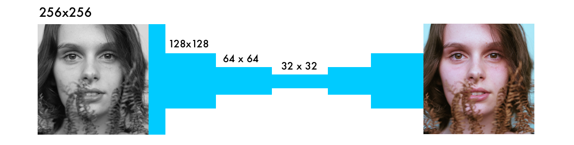
From other neural networks that work with images, ours are different in that the location of pixels is important for it. In coloring neural networks, the image size or aspect ratio remains unchanged. And for other types of networks, the image is distorted as it approaches the final version.
The layer of pooling with the maximum function used in the classifying networks increases the information density, but at the same time distorts the picture. It evaluates information only, not image layout. And in the coloring networks to halve the width and height, we use step 2 (stride of 2). Information density is also increasing, but the picture is not distorted.
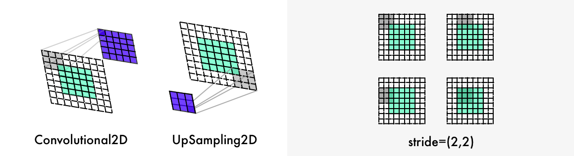
Also, our neural network is different from other layers of upsampling and preserving the aspect ratio of the image. Classifying networks only care about the final classification, so they gradually reduce the size and quality of the image as it runs through the neural network.
Coloring neural networks do not change the aspect ratio of the image. To do this, white fields are added using the parameter
*padding='same'* , as in the illustration above. Otherwise each convolutional layer would cut the images.To double the size of the image, the coloring neural network uses a resampling layer .
for filename in os.listdir('/Color_300/Train/'):
X.append(img_to_array(load_img('/Color_300/Test'+filename)))
This
for-loop first counts the names of all files in the directory, traverses the directory and converts all the pictures into arrays of pixels, and finally merges them into a huge vector.datagen = ImageDataGenerator(
shear_range=0.2,
zoom_range=0.2,
rotation_range=20,
horizontal_flip=True)With the help of ImageDataGenerator, you can turn on the image generator. Then each image will be different from the previous ones, which will speed up learning of the neural network. The
shear_range sets the image tilt to the left or right, it can also be increased, rotated or reflected horizontally.batch_size = 50
def image_a_b_gen(batch_size):
for batch in datagen.flow(Xtrain, batch_size=batch_size):
lab_batch = rgb2lab(batch)
X_batch = lab_batch[:,:,:,0]
Y_batch = lab_batch[:,:,:,1:] / 128
yield (X_batch.reshape(X_batch.shape+(1,)), Y_batch)Apply these settings to the images in the Xtrain folder and generate new images. Then we will extract the black and white layer for
X_batch and two colors for the two color layers.model.fit_generator(image_a_b_gen(batch_size), steps_per_epoch=1, epochs=1000)The more powerful your video card, the more pictures you can process in it simultaneously. For example, the described system can handle 50-100 images. The value of the steps_per_epoch parameter is obtained by dividing the number of training images by the batch size (batch size).
For example: if we have 100 pictures, and the size of the series is 50, then we get 2 stages in the period. The number of periods determines how many times you will train the neural network on all pictures. If you have 10 thousand pictures and 21 periods, then it will take about 11 hours on the Tesla K80 video card.
What have you learned
- First, more experiments with small series, and then you can move on to large runs . We had mistakes even after 20–30 experiments. If something is done, it does not mean that it works. Bugs in neural networks are generally less noticeable than traditional programming errors. For example, one of our most bizarre bugs was Adam hiccup .
- The more diverse dataset, the more brown will be in the images . If your dataset has very similar images , then the neural network will work pretty well without using a more complex architecture. But such a neural network will be worse to generalize.
- Forms, forms and forms again . The size of the images must be accurate and proportional to each other during the entire operation of the neural network. First, we used an image of 300 pixels, then several times we reduced it twice: to 150, 75, and 35.5 pixels. In the last version, half a pixel was lost, which made it necessary to substitute a bunch of crutches, until it came to that it was better to use a deuce to the degree: 2, 4, 8, 16, 32, 64, 256, and so on.
- Creating datasets : a) Disable the .DS_Store file, otherwise it will drive you crazy. b) Show fiction. To download the files, we used the console script in Chrome and the extension . c) Make copies of the source files you are processing and arrange the scripts for cleaning .
Full version of the neural network
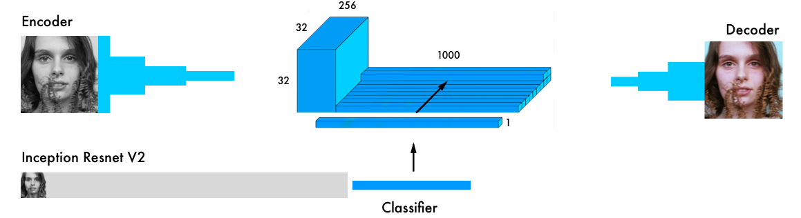
Our final version of the neural network contains four components. We divided the previous network into an encoder and a decoder, and between them a fusion layer. If you are not familiar with the classifying neural networks, we recommend reading this guide: http://cs231n.imtqy.com/classification/ .
Input data simultaneously passes through the encoder and through the most powerful modern classifier - Inception ResNet v2 . This is a neural network trained on 1.2 million images. We extract the classification layer and merge it with the encoder output.
A more detailed visual explanation: https://github.com/baldassarreFe/deep-koalarization .
If you transfer training from the classifier to the coloring network, it will be able to understand what is depicted in the picture, and therefore compare the representation of the object with the coloring scheme.
Here are some test images, only 20 images were used to train the network.

Most of the pictures are crooked. But thanks to a large test set (2500 images), there are some decent ones. Studying the network on a larger sample gives more stable results, but still most of the pictures turned out brown. Here is a complete list of experiments and test images.
The most common architectures from various research projects are:
- Manually add small colored dots to the image to give the network a hint ( link ).
- We find a similar image and transfer colors from it (more here and here ).
- The residual encoder layer and the merging classification layer ( link ).
- We merge hypercolumns from the classifying network (more details here and here ).
- We unite the final classification between the encoder and the decoder (more here and here ).
Color spaces : Lab, YUV, HSV and LUV (more here and here )
Losses : standard error, classification, weighted classification ( link ).
We chose the “merge layer” architecture (fifth on the list) because it gave the best results. It is also easier to understand and easier to reproduce in Keras . Although this is not the strongest architecture, but for the beginning it will fit.
The structure of our neural network is borrowed from the work of Federico Baldasarre and his colleagues, and adapted to work with Keras. Note: In this code, a functional API is used instead of the sequential model Keras. [ Documentation ]
# Get images
X = []
for filename in os.listdir('/data/images/Train/'):
X.append(img_to_array(load_img('/data/images/Train/'+filename)))
X = np.array(X, dtype=float)
Xtrain = 1.0/255*X

#Load weights
inception = InceptionResNetV2(weights=None, include_top=True)
inception.load_weights('/data/inception_resnet_v2_weights_tf_dim_ordering_tf_kernels.h5')
inception.graph = tf.get_default_graph()
embed_input = Input(shape=(1000,))

#Encoder
encoder_input = Input(shape=(256, 256, 1,))
encoder_output = Conv2D(64, (3,3), activation='relu', padding='same', strides=2)(encoder_input)
encoder_output = Conv2D(128, (3,3), activation='relu', padding='same')(encoder_output)
encoder_output = Conv2D(128, (3,3), activation='relu', padding='same', strides=2)(encoder_output)
encoder_output = Conv2D(256, (3,3), activation='relu', padding='same')(encoder_output)
encoder_output = Conv2D(256, (3,3), activation='relu', padding='same', strides=2)(encoder_output)
encoder_output = Conv2D(512, (3,3), activation='relu', padding='same')(encoder_output)
encoder_output = Conv2D(512, (3,3), activation='relu', padding='same')(encoder_output)
encoder_output = Conv2D(256, (3,3), activation='relu', padding='same')(encoder_output)

#Fusion
fusion_output = RepeatVector(32 * 32)(embed_input)
fusion_output = Reshape(([32, 32, 1000]))(fusion_output)
fusion_output = concatenate([encoder_output, fusion_output], axis=3)
fusion_output = Conv2D(256, (1, 1), activation='relu', padding='same')(fusion_output)

#Decoder
decoder_output = Conv2D(128, (3,3), activation='relu', padding='same')(fusion_output)
decoder_output = UpSampling2D((2, 2))(decoder_output)
decoder_output = Conv2D(64, (3,3), activation='relu', padding='same')(decoder_output)
decoder_output = UpSampling2D((2, 2))(decoder_output)
decoder_output = Conv2D(32, (3,3), activation='relu', padding='same')(decoder_output)
decoder_output = Conv2D(16, (3,3), activation='relu', padding='same')(decoder_output)
decoder_output = Conv2D(2, (3, 3), activation='tanh', padding='same')(decoder_output)
decoder_output = UpSampling2D((2, 2))(decoder_output)
model = Model(inputs=[encoder_input, embed_input], outputs=decoder_output)

#Create embedding
def create_inception_embedding(grayscaled_rgb):
grayscaled_rgb_resized = []
for i in grayscaled_rgb:
i = resize(i, (299, 299, 3), mode='constant')
grayscaled_rgb_resized.append(i)
grayscaled_rgb_resized = np.array(grayscaled_rgb_resized)
grayscaled_rgb_resized = preprocess_input(grayscaled_rgb_resized)
with inception.graph.as_default():
embed = inception.predict(grayscaled_rgb_resized)
return embed

# Image transformer
datagen = ImageDataGenerator(
shear_range=0.4,
zoom_range=0.4,
rotation_range=40,
horizontal_flip=True)

#Generate training data
batch_size = 20
def image_a_b_gen(batch_size):
for batch in datagen.flow(Xtrain, batch_size=batch_size):
grayscaled_rgb = gray2rgb(rgb2gray(batch))
embed = create_inception_embedding(grayscaled_rgb)
lab_batch = rgb2lab(batch)
X_batch = lab_batch[:,:,:,0]
X_batch = X_batch.reshape(X_batch.shape+(1,))
Y_batch = lab_batch[:,:,:,1:] / 128
yield ([X_batch, create_inception_embedding(grayscaled_rgb)], Y_batch)

#Train model
tensorboard = TensorBoard(log_dir="/output")
model.compile(optimizer='adam', loss='mse')
model.fit_generator(image_a_b_gen(batch_size), callbacks=[tensorboard], epochs=1000, steps_per_epoch=20)

#Make a prediction on the unseen images
color_me = []
for filename in os.listdir('../Test/'):
color_me.append(img_to_array(load_img('../Test/'+filename)))
color_me = np.array(color_me, dtype=float)
color_me = 1.0/255*color_me
color_me = gray2rgb(rgb2gray(color_me))
color_me_embed = create_inception_embedding(color_me)
color_me = rgb2lab(color_me)[:,:,:,0]
color_me = color_me.reshape(color_me.shape+(1,))

# Test model
output = model.predict([color_me, color_me_embed])
output = output * 128

# Output colorizations
for i in range(len(output)):
cur = np.zeros((256, 256, 3))
cur[:,:,0] = color_me[i][:,:,0]
cur[:,:,1:] = output[i]
imsave("result/img_"+str(i)+".png", lab2rgb(cur))
FloydHub command to run the full version of the neural network:
floyd run --data emilwallner/datasets/colornet/2:data --mode jupyter --tensorboardTechnical explanation
The Keras functional API is great for concatenating or combining several models.
First, download the Inception ResNet v2 neural network and load the weights. Since we will use two models in parallel, we need to determine which ones. This is done in Tensorflow , Keras backend.
inception = InceptionResNetV2(weights=None, include_top=True)
inception.load_weights('/data/inception_resnet_v2_weights_tf_dim_ordering_tf_kernels.h5')
inception.graph = tf.get_default_graph()
Create a series (batch) of the corrected images. Translate them into b / w and run through the Inception ResNet model.
grayscaled_rgb = gray2rgb(rgb2gray(batch))
embed = create_inception_embedding(grayscaled_rgb)
First you need to change the size of the pictures to feed their models. Then, using the preprocessor, we will bring the pixels and values in color to the desired format. Finally, run the images through the Inception network and extract the final model layer.
def create_inception_embedding(grayscaled_rgb):
grayscaled_rgb_resized = []
for i in grayscaled_rgb:
i = resize(i, (299, 299, 3), mode='constant')
grayscaled_rgb_resized.append(i)
grayscaled_rgb_resized = np.array(grayscaled_rgb_resized)
grayscaled_rgb_resized = preprocess_input(grayscaled_rgb_resized)
with inception.graph.as_default():
embed = inception.predict(grayscaled_rgb_resized)
return embed
Let's go back to the generator. For each series we will generate 20 images of the format described below. The Tesla K80 GPU took about an hour. With this model, this video card can generate up to 50 images at a time without any memory problems.
yield ([X_batch, create_inception_embedding(grayscaled_rgb)], Y_batch)This corresponds to the format of our colornet model.
model = Model(inputs=[encoder_input, embed_input], outputs=decoder_output)encoder_inputis transferred to the Encoder model, its output data are then merged in the merge layer with embed_inputin ; the output of the merge is fed to the input of the Decoder model, which returns the resulting data - decoder_output .fusion_output = RepeatVector(32 * 32)(embed_input)
fusion_output = Reshape(([32, 32, 1000]))(fusion_output)
fusion_output = concatenate([fusion_output, encoder_output], axis=3)
fusion_output = Conv2D(256, (1, 1), activation='relu')(fusion_output)In the merge layer, we first layer with 1000 categories (1000 category layer) multiplied by 1024 (32 * 32). So we get from the Inception model 1024 rows of the final layer. The grid 32 x 32 is transferred from a two-dimensional to a three-dimensional representation, with 1000 category pillars (category pillars). The columns are then associated with the encoder model output. We apply a convolutional network with 254 filters and a 1x1 kernel to the final results of the merge layer.
What have you learned
- The terminology in the research papers was frightening . We spent three days looking for a way to implement the “merge model” in Keras. It sounds so complicated that I simply did not want to take on this task, we tried to find tips that would facilitate our work.
- Questions online . There was not a single comment on Keras's Slack channel, and the questions asked on the Stack Overflow were deleted. But when we began to sort out the problem publicly in search of a simple answer, it became clearer to us how to solve this problem.
- Mailing letters . On the forums, you can be ignored, but if you turn to people directly, they will be more responsive. Skype!
- , , . .
- , - , . , , , . . . , Google, “Epoch 1/22”.
What's next
— . , . , . :
- .
- .
- , .
- (amplifier) RGB. , , .
- .
- . , . «».
- FloydHub.
- - woman.jpg ( 400x400 ).
- - Test, FloydHub-. Notebook Test, . 256x256 . , -.
Source: https://habr.com/ru/post/342388/
All Articles