How to discover a million dollars in your AWS account
We recently talked about ways to save more than a million dollars on AWS annual maintenance . Although we talked in detail about various problems and solutions, the most popular question was still: “I know that I spend too much on AWS, but how can we really break up these expenses into understandable parts?”
At first glance, the problem seems rather simple.
You can easily split your AWS expenses by month and finish on it. Ten thousand dollars for EC2, one thousand for S3, five hundred dollars for network traffic, etc. But there is something important missing - the combination of which particular products and development groups accounts for the lion's share of the costs.
')
And note that you can change hundreds of instances and millions of containers. Soon, what at first seemed like a simple analytical problem becomes unimaginably complex.
In this continuation of the article, we would like to share information about the toolkit that we use ourselves. We hope to be able to come up with a few ideas on how to analyze your costs with AWS, regardless of whether you have a couple of instances or tens of thousands.
If you are doing extensive operations on AWS, you probably have two problems already.
Firstly, it is difficult to notice if suddenly one of the development groups suddenly increases its budget.
Our AWS bill exceeds $ 100K per month, and the cost of each AWS component changes rapidly. In each specific week, we can roll out five new services, optimize the performance of DynamoDB and connect hundreds of new customers. In such a situation, it is easy to miss the attention that some one team spent on EC2 by $ 20,000 more than last month.
Secondly, it is difficult to predict how much the cost of servicing new customers will cost.
For clarity, our company Segment offers a single API that sends analytical data to any third-party tools, data warehouses, S3 or internal information systems of companies.
Although customers quite accurately predict how much traffic they will need and what products they prefer to use, but we constantly have problems with translating such a forecast into a specific dollar amount. Ideally, we would like to say: “1 million new API calls will cost us $ X, so we need to make sure we take at least $ Y from the client”.
The solution to this problem for us was the division of infrastructure into what we call “product lines”. In our case, these directions are vaguely formulated as follows:
Analyzing the whole project, we came to the conclusion that it is almost impossible to measure everything . So instead, we set the task of tracking part of the costs in the account, say, 80%, and try to track these costs from beginning to end.
It is more useful for businesses to analyze 80% of the account than to aim at 100%, get bogged down at the data collection stage and never produce any result. Reaching 80% of the costs (the willingness to say “this is enough”) saved us again and again from futile data picking that does not give a dollar of savings.
To split the costs by product, you need to download data for the billing system, that is, collect and subsequently combine the following data:
When we have determined the product directions for all this data, we can upload them for analysis to Redshift.
Analyzing your costs starts with parsing a CSV file from AWS. You can activate the corresponding option on the billing portal - and Amazon will save a CSV file with detailed billing information every day to S3.
By detailed, I mean VERY detailed. Here is a typical line in the report:
This is due to an impressive amount of $ 0.00000001, that is, one millionth cent, for storage in the DynamoDB database of a single table on February 7 between 3:00 and 4:00 o'clock at night. On a typical day, our CSV contains approximately six million such records. ( Unfortunately, most of them are with larger amounts than one millionth cent .)
To transfer data from S3 to Redshift we use the awsdetailedbilling tool from Heroku. This is a good start, but we didn’t have a normal way to link specific AWS costs to our product lines (that is, whether a specific instance time was used for integrations or for data warehouses).
Moreover, approximately 60% of the cost comes from EC2. Although this is the lion's share of costs, it is absolutely impossible to understand the connection between EC2 instances and specific product lines only from the CSV that AWS generates.
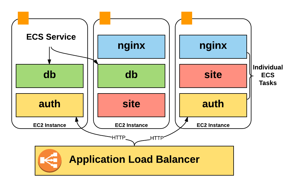
There is an important reason why we couldn’t identify product lines simply by instance name. The fact is that instead of running one process at a host, we use ECS (Elastic Container Service) intensively to place hundreds of containers on a host and use resources much more intensively.
Unfortunately, Amazon accounts only contain EC2 instance costs, so we did not have any information about the costs of containers running on the instance: how many containers were running at the usual time, how much of the pool we used, how many CPU and memory units we used.
Worse, nowhere in the CSV is information about container autoscaling reflected. To obtain this data for analysis, I had to write my own toolkit for collecting information. In the following chapters, I will explain in more detail how this pipeline works.
However, the AWS CSV file provides very good detailed service usage data, which became the basis for the analysis. You just need to connect them with our grocery lines.
Note: This problem is also not going anywhere. Instance-hours billing will become more and more of a concern in terms of “What do I spend my money on?” Because more and more companies are launching a bunch of containers on a large number of instances using systems like ECS, Kubernetes and Mesos. There is some irony in the fact that Amazon itself has been experiencing the exact same problem for many years, because each EC2 instance is a Xen hypervisor that works in conjunction with other instances on the same physical server.
The most important and ready-to-process data comes from AWS “tagged” resources.
By default, billing CSV does not contain any tags. Therefore, it is impossible to distinguish how one EC2 instance or bake behaves compared to another.
However, you can activate some labels that will appear next to your expenses for each unit using the cost allocation tags .
These tags are officially supported by many AWS resources, S3 buckets, DynamoDB tables, etc. To display the cost allocation tags in CSV, you can enable the corresponding parameter in the AWS billing console. After a day or so, the tag you selected (we selected
If you’ve not done any more optimizations, you can immediately start using the cost allocation tags for marking up your infrastructure. This is essentially a “free” service and does not require any infrastructure to operate.
After activating the function, we had two tasks: 1) marking the entire existing infrastructure; 2) checking that all new resources will be automatically tagged.
Tagging for existing infrastructure is pretty easy: for each specific AWS product, you request a list of the most expensive resources in Redshift - and slacken people in Slack until they tell you how to mark these resources. Finish the procedure when tagging 90% or more of the resources by value.
However, to ensure that new resources are flagged, some automation and tools are required.
For this we use Terraform . In most cases, the Terraform configuration supports adding the same cost allocation tags that are added through the AWS console. Here is an example Terraform configuration for S3 Bucket:
Although Terraform provides a basic configuration, we wanted to make sure that every time a new
Fortunately, Terraform configurations are written in HCL (Hashicorp Configuration Language), which has a configuration parser with comments saved. So we wrote a validation function that runs through all Terraform files and searches for markup resources without the
We have established continuous integration for the repository with Terraform configs, and then added these checks, so tests will not pass if there is a resource to be markup without the
This is not ideal — tests are choosy, and people technically have the ability to create unlabeled resources directly in the AWS console, but the system works quite well for this stage. The easiest way to describe a new infrastructure is through Terraform.

After resource markup, their accounting is a simple task.
You may want to break down the costs of AWS services - we have two separate tables, one for the product segments of Segment, and the other for AWS services.
With the usual AWS cost sharing tags, we managed to allocate about 35% of the costs.
This approach is good for marked up, accessible instances. But in some cases, AWS takes an advance payment for "booking." Booking guarantees the availability of a certain amount of resources in exchange for an advance payment at reduced rates.
In our case, it turns out that several large payments from last year’s December CSV account should be distributed over all months of the current year.
To correctly account for these costs, we decided to use data on separate (unblended) costs for the period. The request looks like this:
Subscription costs are recorded in the form of "$ X0000 of DynamoDB", so that they can not be attributed to any resource or product direction.
Instead, we add up the cost of each resource by product line, and then we distribute the cost of the subscription in accordance with the percentage share. If 60% of the expenses of EC2 were spent on data storage, we assume that 60% of the subscription fee for these purposes also went away.
This is also not perfect. If most of your account is taken from an advance payment, this distribution strategy will be distorted by small changes in current expenditures for operating instances. In this case, you will want to distribute expenses based on information on the use of each resource, and it is more difficult to summarize than expenses.
Although the DynamoDB instance and table layout is great, other AWS resources do not support cost sharing tags. These resources required the creation of an abstruse workflow in the style of Ruba Goldberg in order to successfully obtain data on costs and transfer them to Redshift.
The two largest groups of unlabeled resources in our case are ECS and EBS.
The ECS system continuously increases and reduces the scale of our services, depending on the number of containers that each of them needs to work. She is also responsible for rebalancing and packaging in containers in a large number of individual instances.
ECS runs containers on hosts based on the number of "reserved CPUs and memory." Each service tells you how many CPU parts it needs, and ECS either places new containers on the host with enough resources, or scales the number of instances to add the necessary resources.
None of these ECS actions is directly reflected in the CSV billing report - but ECS is still responsible for running autoscaling for all of our instances.
Simply put, we wanted to understand what “part” of a particular machine each container uses, but the CSV report only gives us a breakdown of the “whole unit” by instance.
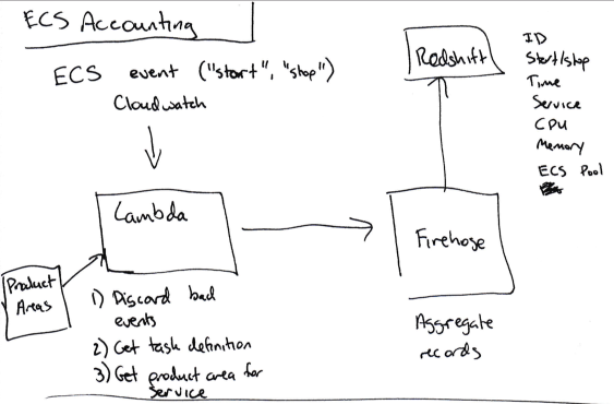
To determine the cost of a particular service, we developed our own algorithm:
As soon as all the start / stop / size data arrived at Redshift, we multiply the amount of time that this task worked in ECS (say, 120 seconds) by the number of CPU units it used on this machine (up to 4096 - this information is available in task description) to calculate the number of CPU-seconds for each service running on the instance.
The total costs of the instance from the account are then divided between the services in accordance with the number of used CPU-seconds.
This is also not an ideal method. EC2 instances do not run all the time at 100% capacity, while the surplus is currently distributed among all services that worked on this instance. This may or may not be the correct allocation of excess costs. But (and here you can find out the general theme of this article) that is enough.
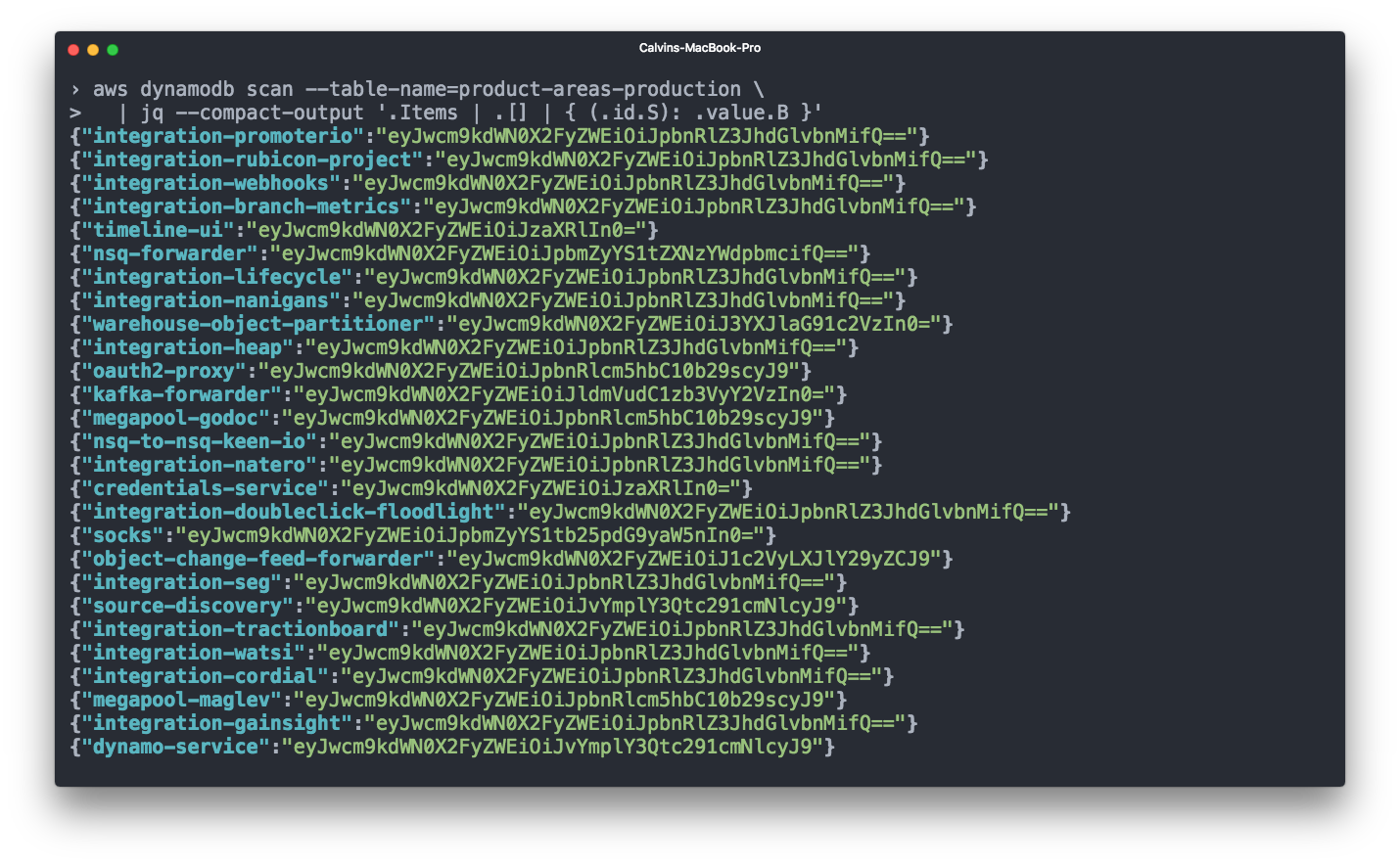
In addition, we want to relate each ECS service to the corresponding product line. However, we cannot mark them in AWS, because ECS does not support cost sharing tags .
Instead, we add the
This script then for each new data transfer publishes to the main branch for DynamoDB a map relating the names of services and product directions in base64 encoding.
Finally, then our tests check every new service that is tagged with the product line.
Elastic Block Storage (EBS) also occupies a significant part of our account. EBS volumes are usually connected to EC2 instances, and it makes sense to consider the costs of EBS volumes together with the corresponding EC2 instances for accounting. However, the CSV billing from AWS does not show which EBS volume is connected to which instance.
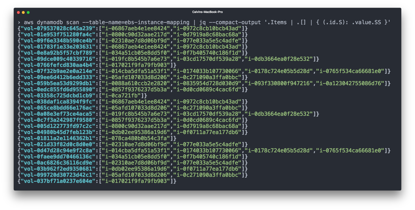
To do this, we again used Cloudwatch - subscribed to events such as “connect volume” and “disconnect volume”, and then registered EBS = EC2 links in the DynamoDB table.
We then add the costs of the EBS volumes to the costs of the corresponding EC2 instances before we consider the costs of the ECS.
So far, we have been discussing all our expenses in the context of a single AWS account. But in reality this does not reflect our real AWS configuration, which is distributed across different AWS physical accounts.
We use an operational account (Ops) not only to consolidate data and billing across all accounts, but also to provide a single point of access for engineers to make changes in production. We separate the Stage stage from the production - so you can check that the API call, for example, to delete the DynamoDB table, is safely handled with the appropriate checks.
Among these expense accounts, the Prod account dominates, but Stage account costs also account for a significant portion of the total AWS account.
Difficulties begin when you need to write data about ECS services from your Stage account to the Redshift cluster on production.
To be able to write “between accounts”, we must allow Cloudwatch subscription handlers to take on production roles for writing to Firehose (for ECS) or DynamoDB (for EBS). This is not easy to do, because you need to add the correct permissions of the correct function in the Stage account (sts.AssumeRole) and in the Prod account, and any error will lead to confusion permissions.
For us, this means that the code for accounting does not work on the Stage account, and all information is entered into the database on the Prod account.
Although a second service can be added to the Stage account, which is subscribed to the same data, but does not record it, we decided that in this case there is a chance to encounter random problems in the accounting code of the Stage.
Finally, we have everything for proper data analysis:
To give it all to the analytic team, I broke the AWS data. For each AWS service, I summarized the Segment product lines and their costs for this AWS service.
These data are given in three different tables:
The total costs for individual product lines look like this:
And the costs of AWS services in combination with the Segment product lines look like this:
For each of these tables, we have a summary table with totals for each month and an additional pivot table that updates the data for the current month every day. The unique identifier in the pivot table matches each pass, so you can consolidate the AWS score by finding all the rows for that pass.
The resulting data effectively serves as our golden "source of truth", which is used for high-level metrics and reporting to management. Pivot tables are used to monitor current costs during the month.
Note: AWS issues a “final” account only a few days after the end of the month, so any logic that marks the billing records as final at the end of the month will be incorrect. You can find out the final Amazon score when an integer appears in the
Before concluding, we realized that in the whole process there are some places where a little preparation and knowledge could save us a lot of time. Without any sorting here are these places:
Getting AWS visuals is not easy. This requires a lot of work — both for developing and configuring the toolkit, and for identifying expensive resources on AWS.
The biggest victory we have achieved is the possibility of simple continuous cost forecasting instead of periodic “one-time analyzes”.
To do this, we automated all data collection, implemented tag support in Terraform and our continuous integration system, and explained to all members of the development team how to tag their infrastructure correctly.
All our data is not dead weight in PDF, but is continuously updated in Redshift. If we want to answer new questions and generate new reports, we instantly get the results using a SQL query.
In addition, we exported all the data in Excel format, where we can accurately calculate how much a new client will cost us. And we can also see if a lot more money suddenly goes to some kind of service or product line - we see it before unplanned expenses affect the financial condition of the company.
, - , !
At first glance, the problem seems rather simple.
You can easily split your AWS expenses by month and finish on it. Ten thousand dollars for EC2, one thousand for S3, five hundred dollars for network traffic, etc. But there is something important missing - the combination of which particular products and development groups accounts for the lion's share of the costs.
')
And note that you can change hundreds of instances and millions of containers. Soon, what at first seemed like a simple analytical problem becomes unimaginably complex.
In this continuation of the article, we would like to share information about the toolkit that we use ourselves. We hope to be able to come up with a few ideas on how to analyze your costs with AWS, regardless of whether you have a couple of instances or tens of thousands.
Grouping by "product lines"
If you are doing extensive operations on AWS, you probably have two problems already.
Firstly, it is difficult to notice if suddenly one of the development groups suddenly increases its budget.
Our AWS bill exceeds $ 100K per month, and the cost of each AWS component changes rapidly. In each specific week, we can roll out five new services, optimize the performance of DynamoDB and connect hundreds of new customers. In such a situation, it is easy to miss the attention that some one team spent on EC2 by $ 20,000 more than last month.
Secondly, it is difficult to predict how much the cost of servicing new customers will cost.
For clarity, our company Segment offers a single API that sends analytical data to any third-party tools, data warehouses, S3 or internal information systems of companies.
Although customers quite accurately predict how much traffic they will need and what products they prefer to use, but we constantly have problems with translating such a forecast into a specific dollar amount. Ideally, we would like to say: “1 million new API calls will cost us $ X, so we need to make sure we take at least $ Y from the client”.
The solution to this problem for us was the division of infrastructure into what we call “product lines”. In our case, these directions are vaguely formulated as follows:
- Integration (code that sends data from Segment to various analytics providers).
- API (a service that receives data in the Segment from client libraries).
- Data warehouses (a pipeline that loads Segment data into a user-defined data store ).
- Website and CDN.
- Internal systems (common logic and support systems for all of the above).
Analyzing the whole project, we came to the conclusion that it is almost impossible to measure everything . So instead, we set the task of tracking part of the costs in the account, say, 80%, and try to track these costs from beginning to end.
It is more useful for businesses to analyze 80% of the account than to aim at 100%, get bogged down at the data collection stage and never produce any result. Reaching 80% of the costs (the willingness to say “this is enough”) saved us again and again from futile data picking that does not give a dollar of savings.
Collection, then analysis
To split the costs by product, you need to download data for the billing system, that is, collect and subsequently combine the following data:
- AWS billing information in CSV format is a CSV that generates AWS with all cost items.
- AWS marked resources are resources that can be marked in billing CSV.
- Unlabeled resources are services like EBS and ECS, which need special data conveyors for marking resource consumption by “product lines”.
When we have determined the product directions for all this data, we can upload them for analysis to Redshift.
1. Billing CSV from AWS
Analyzing your costs starts with parsing a CSV file from AWS. You can activate the corresponding option on the billing portal - and Amazon will save a CSV file with detailed billing information every day to S3.
By detailed, I mean VERY detailed. Here is a typical line in the report:
  record_type |  LineItem
 record_id |  60280491644996957290021401
 product_name |  Amazon DynamoDB
 rate_id |  0123456
 subscription_id |  0123456
 pricing_plan_id |  0123456
 usage_type |  USW2-TimedStorage-ByteHrs
 operation |  StandardStorage
 availability_zone |  us-west-2
 reserved_instance |  N
 item_description |  $ 0.25 per free-of-month
 usage_start_date |  2017-02-07 03:00:00
 usage_end_date |  2017-02-07 04:00:00
 usage_quantity |  6e-08
 blended_rate |  0.24952229400
 blended_cost |  0.00000001000
 unblended_rate |  0.25000000000
 unblended_cost |  0.00000001000
 resource_id |  arn: aws: dynamodb: us-west-2: 012345: table / a-table
 statement_month |  2017-02-01
This is due to an impressive amount of $ 0.00000001, that is, one millionth cent, for storage in the DynamoDB database of a single table on February 7 between 3:00 and 4:00 o'clock at night. On a typical day, our CSV contains approximately six million such records. ( Unfortunately, most of them are with larger amounts than one millionth cent .)
To transfer data from S3 to Redshift we use the awsdetailedbilling tool from Heroku. This is a good start, but we didn’t have a normal way to link specific AWS costs to our product lines (that is, whether a specific instance time was used for integrations or for data warehouses).
Moreover, approximately 60% of the cost comes from EC2. Although this is the lion's share of costs, it is absolutely impossible to understand the connection between EC2 instances and specific product lines only from the CSV that AWS generates.
There is an important reason why we couldn’t identify product lines simply by instance name. The fact is that instead of running one process at a host, we use ECS (Elastic Container Service) intensively to place hundreds of containers on a host and use resources much more intensively.
Unfortunately, Amazon accounts only contain EC2 instance costs, so we did not have any information about the costs of containers running on the instance: how many containers were running at the usual time, how much of the pool we used, how many CPU and memory units we used.
Worse, nowhere in the CSV is information about container autoscaling reflected. To obtain this data for analysis, I had to write my own toolkit for collecting information. In the following chapters, I will explain in more detail how this pipeline works.
However, the AWS CSV file provides very good detailed service usage data, which became the basis for the analysis. You just need to connect them with our grocery lines.
Note: This problem is also not going anywhere. Instance-hours billing will become more and more of a concern in terms of “What do I spend my money on?” Because more and more companies are launching a bunch of containers on a large number of instances using systems like ECS, Kubernetes and Mesos. There is some irony in the fact that Amazon itself has been experiencing the exact same problem for many years, because each EC2 instance is a Xen hypervisor that works in conjunction with other instances on the same physical server.
2. Cost data from AWS marked resources
The most important and ready-to-process data comes from AWS “tagged” resources.
By default, billing CSV does not contain any tags. Therefore, it is impossible to distinguish how one EC2 instance or bake behaves compared to another.
However, you can activate some labels that will appear next to your expenses for each unit using the cost allocation tags .
These tags are officially supported by many AWS resources, S3 buckets, DynamoDB tables, etc. To display the cost allocation tags in CSV, you can enable the corresponding parameter in the AWS billing console. After a day or so, the tag you selected (we selected
product_area ) will begin to appear as a new column next to the corresponding resources in the detailed CSV report.If you’ve not done any more optimizations, you can immediately start using the cost allocation tags for marking up your infrastructure. This is essentially a “free” service and does not require any infrastructure to operate.
After activating the function, we had two tasks: 1) marking the entire existing infrastructure; 2) checking that all new resources will be automatically tagged.
Layout of existing infrastructure
Tagging for existing infrastructure is pretty easy: for each specific AWS product, you request a list of the most expensive resources in Redshift - and slacken people in Slack until they tell you how to mark these resources. Finish the procedure when tagging 90% or more of the resources by value.
However, to ensure that new resources are flagged, some automation and tools are required.
For this we use Terraform . In most cases, the Terraform configuration supports adding the same cost allocation tags that are added through the AWS console. Here is an example Terraform configuration for S3 Bucket:
resource "aws_s3_bucket" "staging_table" { bucket = "segment-tasks-to-redshift-staging-tables-prod" tags { product_area = "data-analysis" # this tag is what shows up in the billing CSV } } Although Terraform provides a basic configuration, we wanted to make sure that every time a new
aws_s3_bucket resource is aws_s3_bucket to the Terraform file, the product_area tag is affixed.Fortunately, Terraform configurations are written in HCL (Hashicorp Configuration Language), which has a configuration parser with comments saved. So we wrote a validation function that runs through all Terraform files and searches for markup resources without the
product_area tag. func checkItemHasTag(item *ast.ObjectItem, resources map[string]bool) error { // looking for "resource" "aws_s3_bucket" or similar t := findS3BucketDeclaration(item) tags, ok := hclchecker.GetNodeForKey(t.List, "tags") if !ok { return fmt.Errorf("aws_s3_bucket resource has no tags", resource) } t2, ok := tags.(*ast.ObjectType) if !ok { return fmt.Errorf("expected 'tags' to be an ObjectType, got %#v", tags) } productNode, ok := hclchecker.GetNodeForKey(t2.List, "product_area") if !ok { return errors.New("Could not find a 'product_area' tag for S3 resource. Be sure to tag your resource with a product_area") } } We have established continuous integration for the repository with Terraform configs, and then added these checks, so tests will not pass if there is a resource to be markup without the
product_area tag.This is not ideal — tests are choosy, and people technically have the ability to create unlabeled resources directly in the AWS console, but the system works quite well for this stage. The easiest way to describe a new infrastructure is through Terraform.
Processing data from cost allocation tags
After resource markup, their accounting is a simple task.
- Find
product_areatags for each resource to match resource identifiers withproduct_areatags. - Add up the cost of all resources.
- Add the cost of product lines and record the result in a pivot table.
SELECT sum(unblended_cost) FROM awsbilling.line_items WHERE statement_month = $1 AND product_name='Amazon DynamoDB'; You may want to break down the costs of AWS services - we have two separate tables, one for the product segments of Segment, and the other for AWS services.
With the usual AWS cost sharing tags, we managed to allocate about 35% of the costs.
Analysis of booked instances
This approach is good for marked up, accessible instances. But in some cases, AWS takes an advance payment for "booking." Booking guarantees the availability of a certain amount of resources in exchange for an advance payment at reduced rates.
In our case, it turns out that several large payments from last year’s December CSV account should be distributed over all months of the current year.
To correctly account for these costs, we decided to use data on separate (unblended) costs for the period. The request looks like this:
select unblended_cost, usage_start_date, usage_end_date from awsbilling.line_items where start_date < '2017-04-01' and end_date > '2017-03-01' and product_name = 'Amazon DynamoDB' and resource_id = ''; Subscription costs are recorded in the form of "$ X0000 of DynamoDB", so that they can not be attributed to any resource or product direction.
Instead, we add up the cost of each resource by product line, and then we distribute the cost of the subscription in accordance with the percentage share. If 60% of the expenses of EC2 were spent on data storage, we assume that 60% of the subscription fee for these purposes also went away.
This is also not perfect. If most of your account is taken from an advance payment, this distribution strategy will be distorted by small changes in current expenditures for operating instances. In this case, you will want to distribute expenses based on information on the use of each resource, and it is more difficult to summarize than expenses.
3. Cost data from unlabeled AWS resources
Although the DynamoDB instance and table layout is great, other AWS resources do not support cost sharing tags. These resources required the creation of an abstruse workflow in the style of Ruba Goldberg in order to successfully obtain data on costs and transfer them to Redshift.
The two largest groups of unlabeled resources in our case are ECS and EBS.
ECS
The ECS system continuously increases and reduces the scale of our services, depending on the number of containers that each of them needs to work. She is also responsible for rebalancing and packaging in containers in a large number of individual instances.
ECS runs containers on hosts based on the number of "reserved CPUs and memory." Each service tells you how many CPU parts it needs, and ECS either places new containers on the host with enough resources, or scales the number of instances to add the necessary resources.
None of these ECS actions is directly reflected in the CSV billing report - but ECS is still responsible for running autoscaling for all of our instances.
Simply put, we wanted to understand what “part” of a particular machine each container uses, but the CSV report only gives us a breakdown of the “whole unit” by instance.
To determine the cost of a particular service, we developed our own algorithm:
- Set up a Cloudwatch subscription for each event when the ECS task starts or stops.
- Send relevant data of this event (service names, CPU / memory usage, start or stop, EC2 instance ID) to Kinesis Firehose (to accumulate individual events).
- Send data from Kinesis Firehose to Redshift.
As soon as all the start / stop / size data arrived at Redshift, we multiply the amount of time that this task worked in ECS (say, 120 seconds) by the number of CPU units it used on this machine (up to 4096 - this information is available in task description) to calculate the number of CPU-seconds for each service running on the instance.
The total costs of the instance from the account are then divided between the services in accordance with the number of used CPU-seconds.
This is also not an ideal method. EC2 instances do not run all the time at 100% capacity, while the surplus is currently distributed among all services that worked on this instance. This may or may not be the correct allocation of excess costs. But (and here you can find out the general theme of this article) that is enough.
In addition, we want to relate each ECS service to the corresponding product line. However, we cannot mark them in AWS, because ECS does not support cost sharing tags .
Instead, we add the
product_area key to the Terraform module for each ECS service. This key does not lead to any metadata sent to AWS, but it fills in a script that reads product_area keys for all services.This script then for each new data transfer publishes to the main branch for DynamoDB a map relating the names of services and product directions in base64 encoding.
Finally, then our tests check every new service that is tagged with the product line.
Ebs
Elastic Block Storage (EBS) also occupies a significant part of our account. EBS volumes are usually connected to EC2 instances, and it makes sense to consider the costs of EBS volumes together with the corresponding EC2 instances for accounting. However, the CSV billing from AWS does not show which EBS volume is connected to which instance.
To do this, we again used Cloudwatch - subscribed to events such as “connect volume” and “disconnect volume”, and then registered EBS = EC2 links in the DynamoDB table.
We then add the costs of the EBS volumes to the costs of the corresponding EC2 instances before we consider the costs of the ECS.
Merging data between accounts
So far, we have been discussing all our expenses in the context of a single AWS account. But in reality this does not reflect our real AWS configuration, which is distributed across different AWS physical accounts.
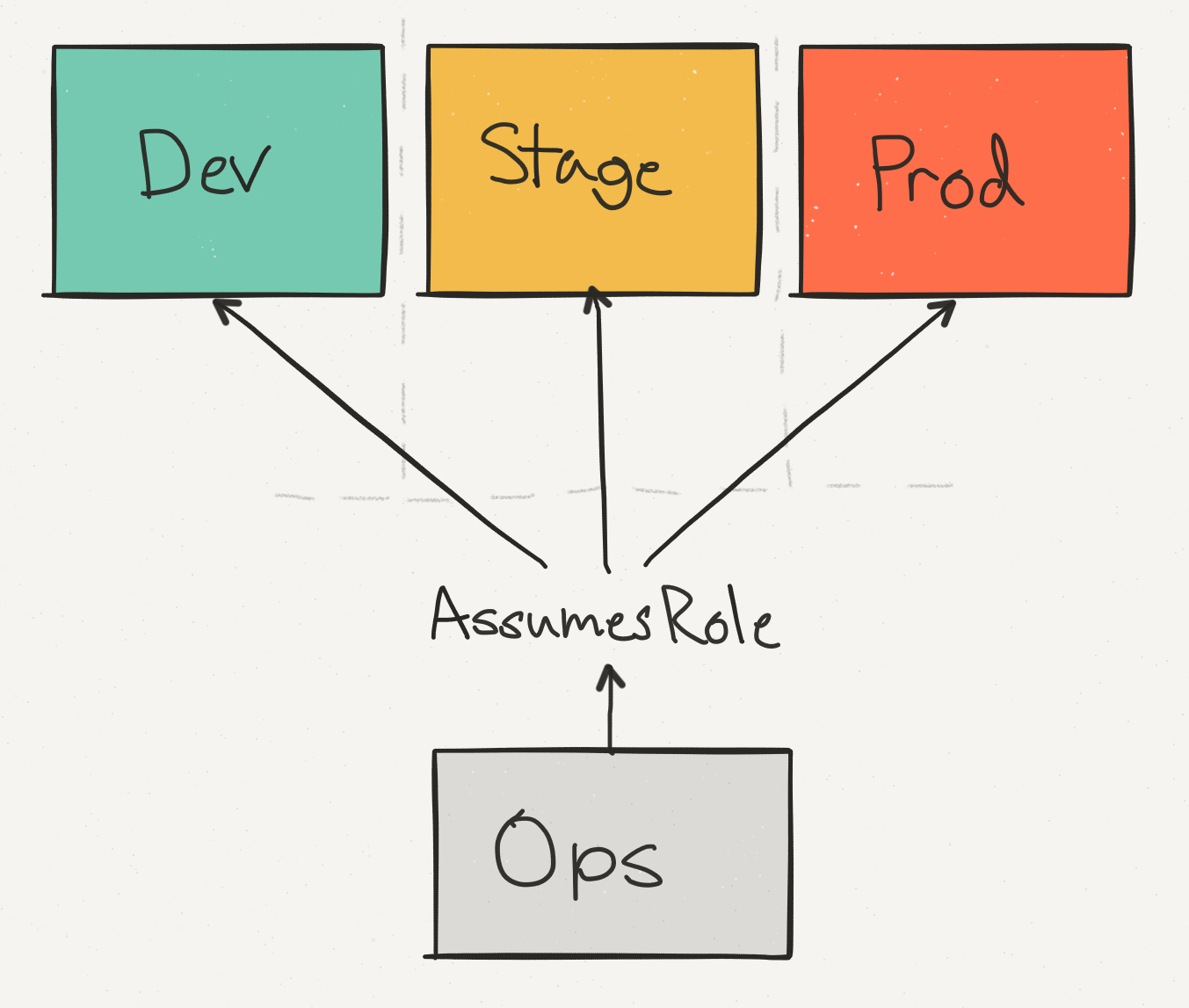
We use an operational account (Ops) not only to consolidate data and billing across all accounts, but also to provide a single point of access for engineers to make changes in production. We separate the Stage stage from the production - so you can check that the API call, for example, to delete the DynamoDB table, is safely handled with the appropriate checks.
Among these expense accounts, the Prod account dominates, but Stage account costs also account for a significant portion of the total AWS account.
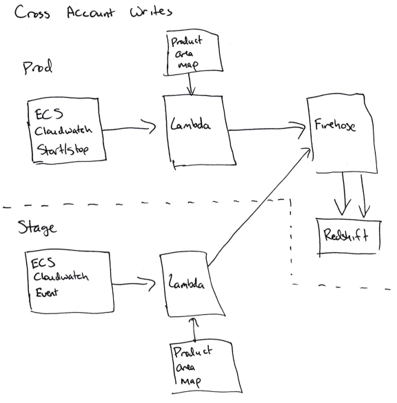
Difficulties begin when you need to write data about ECS services from your Stage account to the Redshift cluster on production.
To be able to write “between accounts”, we must allow Cloudwatch subscription handlers to take on production roles for writing to Firehose (for ECS) or DynamoDB (for EBS). This is not easy to do, because you need to add the correct permissions of the correct function in the Stage account (sts.AssumeRole) and in the Prod account, and any error will lead to confusion permissions.
For us, this means that the code for accounting does not work on the Stage account, and all information is entered into the database on the Prod account.
Although a second service can be added to the Stage account, which is subscribed to the same data, but does not record it, we decided that in this case there is a chance to encounter random problems in the accounting code of the Stage.
Statistics issue
Finally, we have everything for proper data analysis:
- Marked resources in CSV.
- Data when each ECS event starts and stops.
- Binding the names of ECS services to the relevant product lines.
- Binding EBS volumes to connected instances.
To give it all to the analytic team, I broke the AWS data. For each AWS service, I summarized the Segment product lines and their costs for this AWS service.
These data are given in three different tables:
- Total costs for each ECS service in a given month.
- Total expenses for each product line in a given month.
- Total expenses for (AWS service, grocery segment Segment) a given month. For example, "Data Warehouse Direction spent $ 1,000 on DynamoDB last month."
The total costs for individual product lines look like this:
  month |  product_area |  cost_cents
   --------------------------------------
   2017-03-01 |  integrations |  500
   2017-03-01 |  warehouses |  783
And the costs of AWS services in combination with the Segment product lines look like this:
  month |  product_area |  aws_product |  cost_cents
   -------------------------------------------------- -
   2017-03-01 |  integrations |  ec2 |  333
   2017-03-01 |  integrations |  dynamodb |  167
   2017-03-01 |  warehouses |  redshift |  783
For each of these tables, we have a summary table with totals for each month and an additional pivot table that updates the data for the current month every day. The unique identifier in the pivot table matches each pass, so you can consolidate the AWS score by finding all the rows for that pass.
The resulting data effectively serves as our golden "source of truth", which is used for high-level metrics and reporting to management. Pivot tables are used to monitor current costs during the month.
Note: AWS issues a “final” account only a few days after the end of the month, so any logic that marks the billing records as final at the end of the month will be incorrect. You can find out the final Amazon score when an integer appears in the
invoice_id field in the CSV file, not the word “Estimated”.Some last tips
Before concluding, we realized that in the whole process there are some places where a little preparation and knowledge could save us a lot of time. Without any sorting here are these places:
- Scripts that aggregate data or copy it from one place to another are rarely reached by developers — and their work is often not adequately monitored. For example, one of our scripts copied CSV billing data from one S3 bucket to another, but crashed with an error of 27-28 of each month, because the Lambda processor did not have enough memory during copying when the CSV file became large enough. It took us some time to notice this, because Redshift has a lot of data and it looks believable for each month. Since then, we have added monitoring of the Lambda function to ensure the execution of the script without errors.
- Make sure these scripts are well documented, especially with information on how they are involved and what configuration is needed. Link to source code in other places where these scripts are mentioned. For example, in all the places where you are requesting data from bake S3, put a link to a script that writes data to bake. Also think about writing the README file in the S3 batch directory.
- Redshift queries can run really slowly without optimization. Check with your Redshift specialist in your company and think about what queries you need before creating new tables in Redshift. In our case, the correct sort key in the CSV billing tables was missed. After creating the table, you can no longer add sorting keys , so if you do not take care of this in advance, you will have to create a second table with the correct keys, forward write operations there, and then copy all the data.
- Using the correct sort keys reduced the execution time of the query phase during a pass for the pivot table from approximately 7 minutes to 10-30 seconds.
- Initially, we planned to run scripts to update the pivot table on a schedule - Cloudwatch can run the AWS Lambda function several times a day. However, the size of the aisle was inconsistent (especially when it included a record in Redshift) and exceeded the maximum Lambda timeout, so instead we transferred them to the ECS service.
- Initially, we chose JavaScript for the pivot table update code, because it runs on Lambda and most of the scripts in our company are written in JavaScript. If I knew that I would have to switch to ECS, I would choose another language with better support for adding 64-bit numbers, parallelizing and canceling work.
- Every time you start writing new data in Redshift, change the data (say, add new columns) or fix integrity errors with regard to data analysis, add a note to the README file with the date and change information. This will be extremely useful for your data analysis team.
- Blended costs are not very helpful with this type of analysis - stick to unblended costs. They show what specifically AWS charges for this resource.
- The CSV report has 8 or 9 lines, where Amazon does not indicate the name of the service. They represent the total amount of the invoice, but give up any attempts to summarize the unmixed expenses for a given month. Make sure that these figures are excluded from the summation of expenses.
Bottom line
Getting AWS visuals is not easy. This requires a lot of work — both for developing and configuring the toolkit, and for identifying expensive resources on AWS.
The biggest victory we have achieved is the possibility of simple continuous cost forecasting instead of periodic “one-time analyzes”.
To do this, we automated all data collection, implemented tag support in Terraform and our continuous integration system, and explained to all members of the development team how to tag their infrastructure correctly.
All our data is not dead weight in PDF, but is continuously updated in Redshift. If we want to answer new questions and generate new reports, we instantly get the results using a SQL query.
In addition, we exported all the data in Excel format, where we can accurately calculate how much a new client will cost us. And we can also see if a lot more money suddenly goes to some kind of service or product line - we see it before unplanned expenses affect the financial condition of the company.
, - , !
Source: https://habr.com/ru/post/342096/
All Articles