$ mol_app_life: DIY God Simulator

Hello, my name is Dmitry Karlovsky. Recently, I was dying and realized how much I love life. This is an ideal game for sociopaths, where you play the role of God, with your hand unanimously deciding who to live, who to die, and who fallows form. A new cell appears as a result of the intercourse of three other same-sex neighbors and dies being trampled by a crowd of more than three, left alone with themselves or in the company of only one. Who would have thought that such simple laws would generate such a huge variety of gaming experience that they would play Life 50 years after their wording.

If you have not worked with $ mol yet, then it is recommended that you read the " $ mol_app_calc: spreadsheet party " manual, which is more friendly to beginners, before reading. And if you have already mastered it, then you will learn:

How to work with the infinite life field.
How to draw fast vector graphics.
As in $ mol, it is easy and simple to combine control with a finger and drawing graphics.

Vector graphics

$ mol was designed for compactness, code efficiency and ease of use. This means that the application programmer needs only to indicate that where to render without thinking about optimizations, and the graphic modules themselves will figure out how to do it better. The collection of $ mol_plot modules is just such an implementation. In the simplest case, you feed her a vector of numbers and a type of graph, and she herself arranges them as follows:

<= Plot $mol_plot_pane graphs / <= Trend $mol_plot_line series <= trend / 1 2 5 4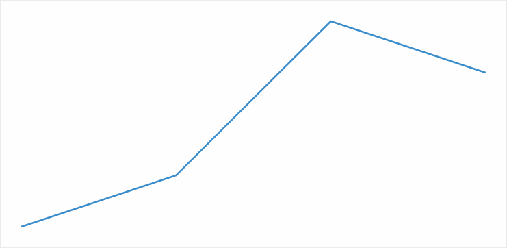

Line graph

The following types are currently supported: linear, columnar, point, and potting. Plus vertical and horizontal rulers. In addition, if a special type of graphics allows you to combine several other types into one, which allows you to design new types of graphs, combining existing ones. For example, we can construct a “Rope type of a graph with a filling”:

 $my_plot_rope $mol_plot_group graphs / <= Line $mol_plot_line <= Dot $mol_plot_dot <= Fill $mol_plot_fill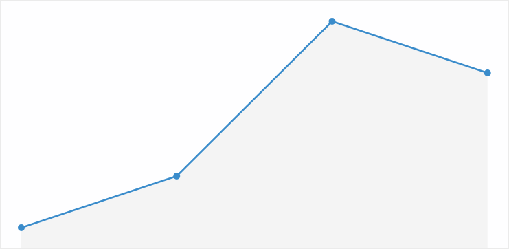

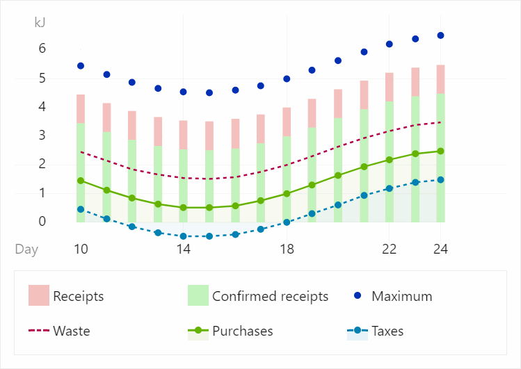
Rope chart

Of course, we can also draw several graphs for different vectors, while $ mol_plot_pane is able to give each graph a unique color starting from the base hue:

 <= Plot $mol_plot_pane hue_base 206 graphs / <= Fact $mol_plot_bar series <= fact / 1000 2000 4000 9000 <= Plan $mol_plot_line series <= plan / 1000 3000 5000 7000 type \dashed

Plan fact

But that's not all, the types of graphs can return samples for the legend. In this case, the samples, as well as the actual graphics, can be combined. So you will never have bugs when one type of line is displayed on the chart, and another in the legend. Just look at the legend automatically generated from the charts:

Graphics speed

The implementation of graphs is not only very compact, but also very effective:

Benchmark rope diagrams

Benchmark bar graphs

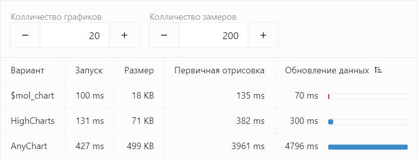
Such efficiency is achieved due to many factors:

Implementation is trite simpler and requires less overhead.
Reactive Programming is used to effectively update states. It is so efficient that you can easily change any aspect of real-time rendering with almost no load on the system. For example: graphic disco .
Points located visually indistinguishably close to each other collapse into one. No matter how much data you put into rendering, it will not fail to put the system in multiple rendering of the same pixel.
Points that fall outside the viewport are excluded from rendering. Actual when panning huge amounts of data. The less we render, the faster we render.
Graphics are drawn with a minimum of SVG elements.

For the last point, there is even a separate benchmark, showing that a properly implemented SVG chart, with rendering an element through one path instead of a heap of line elements, is not much slower than manual rendering on canvas:

SVG vs Canvas

Life Graphics

We will need to draw points that are not arranged in order from left to right, but in arbitrary places. To do this, we will specify not series , but points_raw , which returns not a vector of numbers, but a vector from the coordinates:

 $mol_app_life_map $mol_plot_pane gap 0 graphs / <= Points $mol_plot_dot threshold 0 points_raw <= points /

Please note that we have removed the indents of the graphics from the edge of the rendering area ( gap ) and the collapse of closely spaced points ( threshold ) as we do not need them.

$mol_plot_pane has shift and scale properties allowing centrally changing the size and position of graphs. Let's enter the zoom property, which will set the scaling factor, and pan which will be an alias for shift . Both will be changeable.

 $mol_app_life_map $mol_plot_pane gap 0 - pan?val / 0 0 zoom?val 16 scale / <= zoom - <= zoom - shift <= pan - - graphs / <= Points $mol_plot_dot threshold 0 diameter <= zoom - points_raw <= points /

Please note that we have indicated the diameter of the points equal to the degree of approximation. And by default, the degree of approximation is 16. So the entire field initially will have a 16-pixel grid in our cells which will contain 16-pixel circles.

Zoom and pan

In $ mol there are special components that are not intended for self-rendering, but for adding functionality to others. One of these plugins is $ mol_touch , which intercepts finger and mouse input events and implements various gestures. We only need to change the size of the cells and move the field, so we add a plugin and proving the previously declared properties:

 plugins / <= Touch $mol_touch zoom?val <=> zoom?val - pan?val <=> pan?val -

That's all. True. Bilateral binding is just a wonderful thing. You write a minimum of code, but at the same time everything is under your complete control. When any nested component requests the value of a property or tries to write something into it, your function is called. For example, let's set a minimum approximation level equal to one:

 @ $mol_mem zoom( next = super.zoom() ) { return Math.max( 1 , next ) }

And as the default offset, let's set half the size of the rendering area so that the cell with coordinates [0,0] initially located in the center:

 @ $mol_mem pan( next? : number[] ) { return next || this.size_real().map( v => v / 2 ) }

Rules of the game

It could be limited to a small field in the size of the screen, but we are not looking for easy ways, so our field will be infinite. Well, as infinite ... toroidal, but very large: 64K * 64K = 4G cells.

To calculate the state of each cell of such a huge field is too long an operation. Note that the number of living cells is incomparably smaller than the dead ones. This means that at each step it makes sense to update the state of only living cells and their immediate surroundings.

To do this, we need a structure called Set for storing the coordinates of living cells. But the trouble is that the coordinates of the cell are two numbers, and the key of the set can be only one primitive value (or an object reference, but this is actually also a primitive).

We could serialize numbers into strings and concatenate them with the key. But working with strings is not a quick operation. The most effective is to combine 2 numbers into one using bit operations. Bit operations in JS always result in numbers to a 32-bit representation. So for each coordinate we will have as many as 16 bits - hence the limit on the field size of 4 gigaclets.

Connecting numbers is very simple - we cut to 16 bits and combine them with different offsets:

 function key( a : number , b : number ) { return a << 16 | b & 0xFFFF }

We also need to separate them and to iterate over the set to get the coordinates. It is not difficult to get the higher number just by moving it with the filling with the high bit:

 function x_of( key : number ) { return key >> 16 }

But to get a lower number it is not enough just to trim the high bits, because then the negative values will break, the high bits of which should be ones, not zeros. You need to move the lower bits to the place of the elders, and then the task is reduced to the previous one:

 function y_of( key : number ) { return key << 16 >> 16 }

Now we can create sets and add / remove coordinates from them:

 const state = new Set<[ number , number ]>() state.add( key( 1, 2 ) ) state.add( key( 3, 4 ) ) state.delete( key( 1, 4 ) ) for( let key of state ) { console.log( x_of( key ) , y_of( key ) ) }

Let's get the state reactive property that will keep the state of the universe at the current moment and let it form a multitude of living cells based on the snapshot serialized view through which it will be possible to establish the initial state from the outside:

 @ $mol_mem state( next? : Set<number> ) { const snapshot = this.snapshot() if( next ) return next return new Set( snapshot.split( '~' ).map( v => parseInt( v , 16 ) ) ) }

Please note that we first read the current snapshot, and only then allow it to be overridden. This is necessary so that even if we change the state, it would still be synchronized with the snapshot.

In addition, let us provide the ability to reactively obtain from the component a snapshot of the current altered state:

 @ $mol_mem snapshot_current() { return [ ... this.state() ].map( key => key.toString( 16 ) ).join( '~' ) }

Do not forget to declare the communication properties in view.tree:

 snapshot \ snapshot_current \ - speed 0 population 0

At the same time, we declared the speed property that specifies the frequency of the world update and the population that allows to get the number of living cells at the moment. The latter is easy to implement:

 @ $mol_mem population() { return this.state().size }

Finally, the most interesting thing is to update the state at a given speed. To do this, we will add the future property, which will read the state, on its basis, calculate the new and write back:

 @ $mol_mem future( next? : Set<number> ) { let prev = this.state() const state = new Set<number>() //  state   prev return this.state( state ) }

This property will be calculated once and for all, but we need to periodically, so we add to it a dependence on the current time with the desired frequency:

 @ $mol_mem future( next? : Set<number> ) { let prev = this.state() if( !this.speed() ) return prev this.$.$mol_state_time.now( 1000 / this.speed() ) const state = new Set<number>() //  state   prev return this.state( state ) }

Now it will be disabled every N milliseconds (from 16 to 1000), which will lead to the execution of the method and the updating of the state of the world. By the way, here is the code for this update:

 const state = new Set<number>() const skip = new Set<number>() for( let alive of prev ) { const ax = x_of( alive ) const ay = y_of( alive ) for( let ny = ay - 1 ; ny <= ay + 1 ; ++ny ) for( let nx = ax - 1 ; nx <= ax + 1 ; ++nx ) { const nkey = key( nx , ny ) if( skip.has( nkey ) ) continue skip.add( nkey ) let sum = 0 for( let y = -1 ; y <= 1 ; ++y ) for( let x = -1 ; x <= 1 ; ++x ) { if( !x && !y ) continue if( prev.has( key( nx + x , ny + y ) ) ) ++sum } if( sum != 3 && ( !prev.has( nkey ) || sum !== 2 ) ) continue state.add( nkey ) } }

There are already applied the main optimization. Perhaps you can optimize it even more. Dare!

Finally, create a list of points for rendering:

 points() { const points = [] as number[][] for( let key of this.future().keys() ) { points.push([ x_of( key ) , y_of( key ) ]) } return points }

Divine hand

To make the player not just a mute witness, but a ruler of destinies, we will subscribe to several pointer events:

 event * ^ mousedown?event <=> draw_start?event null mouseup?event <=> draw_end?event null

Despite the name, they work with both the mouse and the finger. Unfortunately, the click event will not work here, because it works even when panning, which we absolutely do not need. Therefore, when the pointer is activated, we will memorize its current position:

 @ $mol_mem draw_start_pos( next? : number[] ) { return next } draw_start( event? : MouseEvent ) { this.draw_start_pos([ event.pageX , event.pageY ]) }

And by deactivating, check the displacement and, if it has not changed much, initiate the switching of the life and death of the cell that came to hand:

 draw_end( event? : MouseEvent ) { const start_pos = this.draw_start_pos() const pos = [ event.pageX , event.pageY ] if( Math.abs( start_pos[0] - pos[0] ) > 4 ) return if( Math.abs( start_pos[1] - pos[1] ) > 4 ) return const zoom = this.zoom() const pan = this.pan() const cell = key( Math.round( ( event.offsetX - pan[0] ) / zoom ) , Math.round( ( event.offsetY - pan[1] ) / zoom ) , ) const state = new Set( this.state() ) if( state.has( cell ) ) state.delete( cell ) else state.add( cell ) this.state( state ) }

Management interface

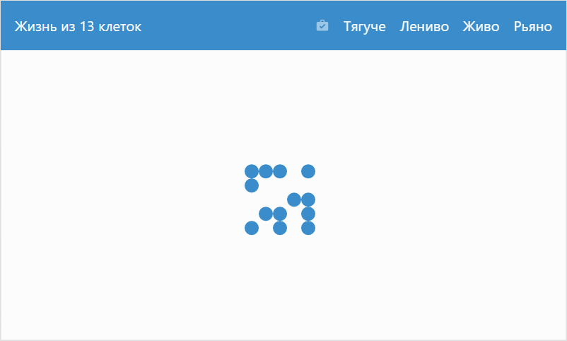
The game field $mol_app_life_map ready, you can start creating an application for managing it. Presenting it from us will be a regular $ mol_page page, consisting of a cap and a playing field:

 $mol_app_life $mol_page title @ \Life of {population} cells sub / <= Head - <= Map $mol_app_life_map speed <= speed - snapshot <= snapshot \ snapshot_current => snapshot_current population => population

Here we set the field speed and basic snapshot, and draw the number of living cells and snepshot of the current state.

In the header, we replace the placeholder with a specific number of living cells:

 title() { return super.title().replace( '{population}' , `${ this.population() }` ) }

Base snapshot we take from the link:

 snapshot() { return this.$.$mol_state_arg.value( 'snapshot' ) || super.snapshot() }

At the same time we form a link to the current state of the world, the transition to which will add the current snapshot to the browser history:

 store_link() { return this.$.$mol_state_arg.make_link({ snapshot : this.snapshot_current() }) }

We will display this link to the toolbar in the header with the speed switch:

 tools / <= Store_link $mol_link uri <= store_link?val \ hint <= store_link_hint @ \Store snapshot sub / <= Stored $mol_icon_stored <= Time $mol_switch value?val <=> speed?val 0 options * 1 <= time_slowest_label @ \Slowest 5 <= time_slow_label @ \Slow 25 <= time_fast_label @ \Fast 60 <= time_fastest_label @ \Fastest

If the link leads to the current snapshot, then we grab it:

 [mol_app_life_store_link][mol_link_current] { opacity: .5; }

And the final touch - add localization:

 { "$mol_app_life_title": "  {population} ", "$mol_app_life_store_link_hint": " ", "$mol_app_life_time_slowest_label": "", "$mol_app_life_time_slow_label": "", "$mol_app_life_time_fast_label": "", "$mol_app_life_time_fastest_label": "" }