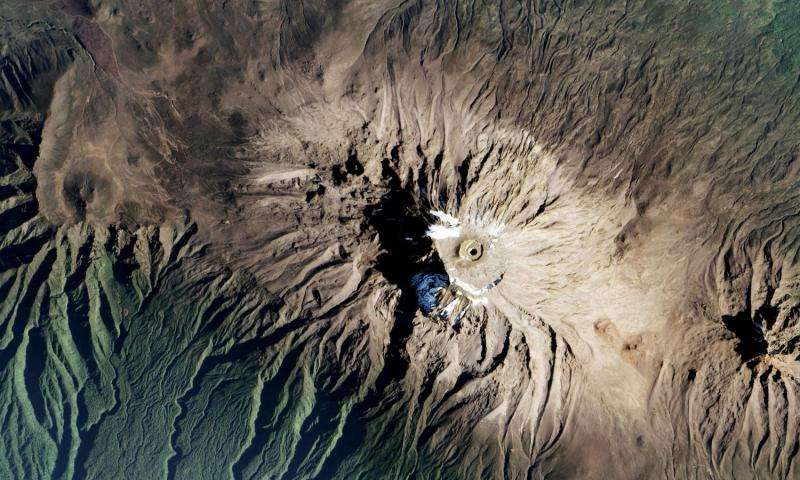
Space photography of the Earth

Satellite image in false colors (green, red, near infrared) with a spatial resolution of 3 meters and superimposed mask of buildings from OpenStreetMap (satellite constellation PlanetScope)

Hi, Habr! We are constantly expanding the sources of data that we use for analytics, so we decided to add more satellite imagery. We have satellite imagery analytics useful in business and investment products. In the first case, statistics on geo-data will help to understand where to open retail outlets, in the second case, it allows analyzing the activities of companies. For example, for construction companies, one can calculate how many floors were built in a month, for agricultural companies, how many hectares of crop have grown, etc.

In this article I will try to give a rough idea of ​​the space imagery of the Earth, talk about the difficulties that can be encountered when starting work with satellite imagery: preliminary processing, algorithms for analysis and the Python library for working with satellite imagery and geodata. So everyone who is interested in the field of computer vision, welcome under the cat!

So, let us begin with the spectral regions in which the satellites perform the survey, and consider the characteristics of the imaging equipment of some satellites.
')

Spectral signatures, atmospheric windows and satellites

Different terrestrial surfaces have different spectral signatures. For example, fresh basaltic lava and asphalt reflect different amounts of infrared light, although they are similar in visible light.


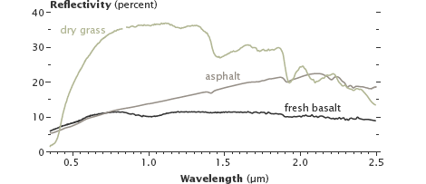
Reflectivity of dry grass, asphalt and fresh basalt lava

Like the surface of the Earth, gases in the atmosphere also have unique spectral signatures. Moreover, not every radiation passes through the atmosphere of the Earth. The spectral ranges passing through the atmosphere are called “atmospheric windows”, and satellite sensors are configured to measure in these windows.


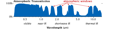
Atmospheric windows

Consider a satellite with one of the highest spatial resolutions - WorldView-3 (Spatial resolution is a quantity characterizing the size of the smallest objects visible in the image; nadir is the direction coinciding with the direction of gravity at that point).

WorldView-3 imaging equipment specifications

Spectral range	Name	Range, nm	Spatial resolution in nadir, m
Panchromatic (1 channel; covers the visible part of the spectrum)		450-800	0.31
Multispectral (8 channels)	Coastal	400-450	1.24
	Blue	450-510
	Green	510-580
	Yellow	585-625
	Red	630-690
	Red edge	705-745
	Near infrared	770-895
	Near infrared	860-1040
Multiband in the short infrared range (8 channels)	SWIR-1	1195-1225	3.70
	SWIR-2	1550-1590
	SWIR-3	1640-1680
	SWIR-4	1710-1750
	SWIR-5	2145-2185
	SWIR-6	2185-2225
	SWIR-7	2235-2285
	SWIR-8	2295-2365

In addition to the above channels, WorldView-3 has 12 more channels designed specifically for atmospheric correction - CAVIS (Clouds, Aerosols, Vapors, Ice, and Snow) with a resolution of 30 m in the nadir and wavelengths from 0.4 to 2.2 microns.


Sample image from WorldView-2; panchromatic channel


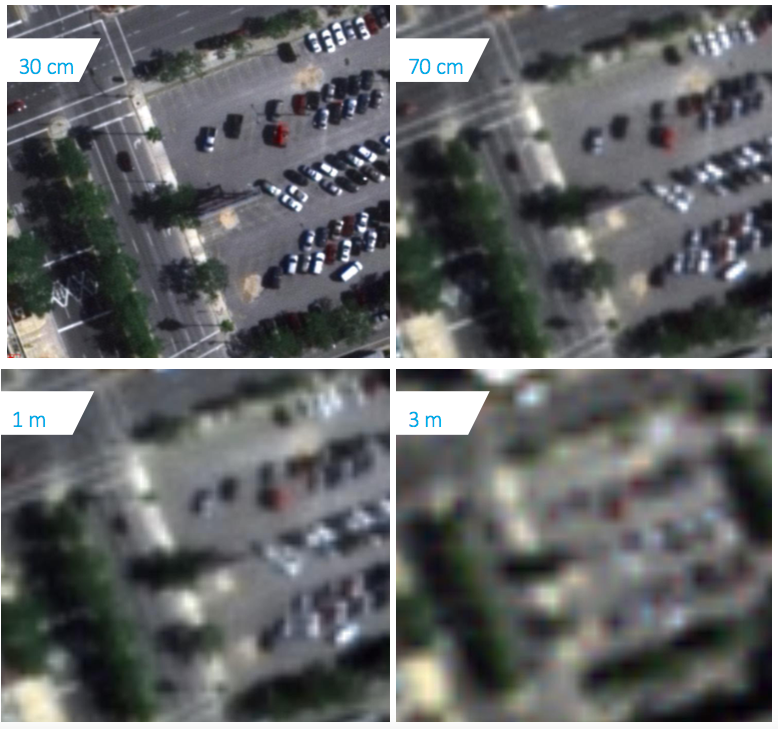
Sample images with different spatial resolution

Other interesting satellites are SkySat-1 and its twin SkySat-2. They are interesting because they are able to shoot video up to 90 seconds over one territory with a frequency of 30 frames / sec and a spatial resolution of 1.1 m.


SkySat satellite footage

The spatial resolution of the panchromatic channel is 0.9 m, multispectral channels (blue, green, red, near infrared) - 2 m.

Some more examples:

1. The grouping of satellites PlanetScope performs shooting with a spatial resolution of 3 m in the red, green, blue and near infrared range;
   
2. The grouping of RapidEye satellites performs surveys with a spatial resolution of 5 m in red, extreme red, green, blue and near infrared;
   
3. A series of Russian satellites "Resurs-P" performs a survey with a spatial resolution of 0.7-1 m in the panchromatic channel, 3-4 m in multispectral channels (8 channels).
   

Unlike multispectral sensors, hyperspectral sensors divide the spectrum into many narrow ranges (approximately 100–200 channels) and have a spatial resolution of a different order: 10–80 m.

Hyperspectral imagery is not as widely available as multispectral imagery. There are few spacecraft equipped with hyperspectral sensors on board. Among them, Hyperion aboard NASA EO-1 satellite (decommissioned), CHRIS aboard PROBA satellite owned by the European Space Agency, FTHSI aboard the MightySatII satellite of the research laboratory of the US Air Force, GSA (hyperspectral apparatus) on Russian space vehicles " Resource-P.


The processed hyperspectral image from the onboard CASI 1500 sensor; up to 228 channels; spectral range 0.4 - 1 nm


Processed image from the space sensor EO-1; 220 channels; spectral range 0.4 - 2.5 nm

To simplify work with multichannel snapshots, there are libraries of pure materials. They show the reflectivity of pure materials.

Pre-processing of images

Before proceeding with the analysis of images, you must perform their preliminary processing:

1. Geolocation;
   
2. Orthocorrection;
   
3. Radiometric correction and calibration;
   
4. Atmospheric correction.
   

Suppliers of satellite imagery take additional measurements to pre-process imagery, and can issue both processed images and raw ones with additional information for self-correction.

It is also worth mentioning the color correction of satellite images - bringing the image in natural colors (red, green, blue) to a more familiar sight for a person.

Approximate geolocation is calculated by the initial position of the satellite in orbit and image geometry. Geo-referencing is performed using ground control points (GCP). These control points are searched on the map and on the image, and knowing their coordinates in different coordinate systems, one can find the transformation parameters (conformal, affine, perspective or polynomial) from one coordinate system to another. GCP search is performed using GPS surveys . 1 sec. 230, exp. 2 ] or by comparing two images, one of which accurately shows the coordinates of the GCP, at key points .

Image orthocorrection is a process of geometric correction of images, which eliminates perspective distortions, reversals, distortions caused by lens distortion and others. In this case, the image is reduced to a planned projection, that is, one in which each point of the terrain is observed strictly vertically, into the nadir.

Since the satellites are shooting from a very high altitude (hundreds of kilometers), then when shooting in the nadir, the distortion should be minimal. But the spacecraft can not shoot all the time in the nadir, otherwise it would take a very long time to wait for the moment when it passes over a given point. To eliminate this drawback, the satellite is “turned over”, and most of the frames are promising. It should be noted that the angles of shooting can reach 45 degrees, and at high altitude this leads to significant distortions.

Orthocorrection should be carried out if measuring and positional properties of the image are needed, since image quality due to additional operations will deteriorate. It is performed by reconstructing the geometry of the sensor at the time of registration for each line of the image and the representation of the relief in raster form.

A satellite camera model is represented as generalized approximating functions (rational polynomials — RPC coefficients), and altitude data can be obtained from ground-based measurements, using contour lines from a topographic map, stereo, radar data, or from commonly available coarse digital elevation models: SRTM ( resolution 30-90 m) and ASTER GDEM (resolution (15-90 m).

Radiometric correction - correction at the stage of preliminary preparation of images of hardware radiometric distortion, due to the characteristics of the used shooting device.

For scanner imaging devices, such defects are observed visually as image modulation (vertical and horizontal stripes). Radiometric correction also removes image defects observed as failed image pixels.


Remove bad pixels and vertical bars

Radiometric correction is performed by two methods:

1. C using known parameters and settings of the shooting device (correction tables);
   
2. Statistically.
   

In the first case, the necessary correction parameters are determined for the imaging instrument based on long-term ground and flight tests. The correction by statistical method is performed by identifying the defect and its characteristics directly from the image itself, subject to correction.

Radiometric calibration of images - transfer of “raw values” of brightness to physical units, which can be compared with the data of other images:

$$

$$B_ \ lambda = K_ \ lambda \; \ ast \; DN_ \ lambda + \; C_ \ lambda,$$

Where $$$B_ \ lambda$- energy brightness for the spectral zone $$$\ lambda$;
$$$DN_ \ lambda$- raw brightness values;
$$$K_ \ lambda$- calibration coefficient;
$$$C_ \ lambda$- calibration constant.

Electromagnetic radiation of the satellite, before it is recorded by the sensor, will pass through the atmosphere of the Earth twice. There are two main effects of the atmosphere - scattering and absorption. Scattering occurs when particles and gas molecules in the atmosphere interact with electromagnetic radiation, deflecting it from the original path. When absorbed, a part of the radiation energy is converted into the internal energy of absorbing molecules, as a result of which the atmosphere is heated. The effect of scattering and absorption on electromagnetic radiation changes as one passes from one part of the spectrum to another.


Factors affecting the incidence of reflected solar radiation on satellite sensors

There are various algorithms for performing atmospheric correction (for example , the Dark Object Subtraction DOS method ). The input parameters for the models are: the geometry of the location of the Sun and the sensor, the atmospheric model for gaseous components, the aerosol model (type and concentration), the optical thickness of the atmosphere, the surface reflection coefficient and spectral channels.
For atmospheric correction, you can also apply the algorithm to remove the haze from the image - Single Image Haze Removal Using Dark Channel Prior ( implementation ).


Work Example Single Image Haze Removal Using Dark Channel Prior

Index Images

When studying objects using multichannel images, it is often not the absolute values ​​that are important, but the characteristic relationships between the brightness values ​​of the object in different spectral zones. To do this, build the so-called index images. In such images, the sought-after objects are more vividly and vividly highlighted in comparison with the original image.

Examples of index images

Index name	Formula	Application
Iron Oxide Index	Red Blue	To detect the content of iron oxides
Clay Minerals Index	The ratio of the brightness values ​​within the middle infrared channel (CIC). CIC1 / CIC2, where CIC1 is the range from 1.55 to 1.75 microns, CIC2 is the range from 2.08 to 2.35 microns	To identify the content of clay minerals
Ferrous Minerals Index	The ratio of the brightness value in the average infrared (SIK1; from 1.55 to 1.75 μm) channel to the brightness value in the near infrared channel (BIC). SIK1 / BIK	To detect glandular minerals
Redness Index (RI)	Based on the difference in reflectivity of red minerals in the red (K) and green (W) ranges. RI = ( - ) / ( + )	To detect the content of iron oxide in the soil
Normalized differential snow index (NDSI)	NDSI is a relative value characterized by the difference in snow reflectivity in the red (K) and shortwave infrared (CIR) ranges. NDSI = (K - KIK) / (K + KIK)	Used to highlight areas covered with snow. For snow NDSI> 0.4
Water Index (WI)	WI = 0.90 µm / 0.97 µm	It is used to determine the water content in vegetation from hyperspectral images
Normalized Differential Vegetation Index (NDVI)	Chlorophyll of plant leaves reflects radiation in the near infrared (NIR) range of the electromagnetic spectrum and absorbs it in red (K). The ratio of brightness values ​​in these two channels allows you to clearly separate and analyze plant from other natural objects. NDVI = (BIK - K) / (BIK + K)	Shows the presence and condition of vegetation. NDVI values ​​range from -1 to 1; Dense vegetation: 0.7; Sparse vegetation: 0.5; Open soil: 0.025; Clouds: 0; Snow and ice: -0.05; Water: -0.25; Artificial materials (concrete, asphalt): -0.5

Working with satellite imagery in Python

One of the formats in which it is customary to store satellite images is GeoTiff (we confine ourselves only to them). To work with GeoTiff in Python, you can use the gdal library or rasterio .

To install gdal and rasterio it is better to use conda:

conda install -c conda-forge gdal conda install -c conda-forge rasterio 

Other libraries for working with satellite images are easily installed via pip.

Reading GeoTiff via gdal:

 from osgeo import gdal import numpy as np src_ds = gdal.Open('image.tif') img = src_ds.ReadAsArray() #height, width, band img = np.rollaxis(img, 0, 3) width = src_ds.RasterXSize height = src_ds.RasterYSize gt = src_ds.GetGeoTransform() #    minx = gt[0] miny = gt[3] + width*gt[4] + height*gt[5] maxx = gt[0] + width*gt[1] + height*gt[2] maxy = gt[3] 

The coordinate systems for satellite images are quite a few. They can be divided into two groups: geographical coordinate systems (GCS) and flat coordinate systems (UCS).

In HSC, units of measurement are angular and coordinates are represented by decimal degrees. The most famous GSK is WGS 84 (EPSG: 4326).

In UCS, units of measure are linear and coordinates can be expressed as meters, feet, kilometers, etc., so they can be interpolated linearly. For the transition from GSK to UCS apply map projections. One of the most famous projections is the Mercator projection.

It is customary to store the map (image markup) not in raster form, but in the form of points, lines and polygons. The geocoordinates of the vertices of these geometric objects are stored inside the files with the markup of the images. You can use the fiona and shapely libraries to read and work with them.

Script for rasterizing polygons:

 import numpy as np import rasterio #fiona       ,  shp  geojson import fiona import cv2 from shapely.geometry import shape from shapely.ops import cascaded_union from shapely.ops import transform from shapely.geometry import MultiPolygon def rasterize_polygons(img_mask, polygons):   if not polygons:       return img_mask     if polygons.geom_type == 'Polygon':       polygons = MultiPolygon([polygons])     int_coords = lambda x: np.array(x).round().astype(np.int32)   exteriors = [int_coords(poly.exterior.coords) for poly in polygons]   interiors = [int_coords(pi.coords) for poly in polygons                for pi in poly.interiors]     cv2.fillPoly(img_mask, exteriors, 255)   cv2.fillPoly(img_mask, interiors, 0)   return img_mask def get_polygons(shapefile):     geoms = [feature["geometry"] for feature in shapefile]   polygons = list()   for g in geoms:           s = shape(g)           if s.geom_type == 'Polygon':               if s.is_valid:                   polygons.append(s)               else:                   #                     polygons.append(s.buffer(0))           elif s.geom_type == 'MultiPolygon':               for p in s:                   if p.is_valid:                       polygons.append(p)                   else:                       #                         polygons.append(p.buffer(0))   mpolygon = cascaded_union(polygons)     return mpolygon #   geojson    src = rasterio.open('image.tif') shapefile = fiona.open('buildings.geojson', "r") #  (      ) left = src.bounds.left right = src.bounds.right bottom = src.bounds.bottom top = src.bounds.top height,width = src.shape #  mpolygon = get_polygons(shapefile) #    ,          mpolygon = transform(lambda x, y, z=None: (width * (x - left) / float(right - left),\                                                      height - height * (y - bottom) / float(top - bottom)), mpolygon) #  real_mask = np.zeros((height,width), np.uint8) real_mask = rasterize_polygons(real_mask, mpolygon) 

While decrypting images, you may need to intersect polygons (for example, automatically marking buildings on a map, you also want to automatically remove the markings of buildings in those places where there are clouds). There is a Wyler-Atherton algorithm for this, but it only works with polygons without self-intersections. To eliminate self-intersections, you need to check the intersection of all edges with other edges of the polygon and add new vertices. These vertices will divide the corresponding edges into parts. The shapely library has a method for eliminating self-intersections - buffer (0).

To translate from GSK to PSK, you can use the PyProj library (or do it in rasterio):

 #      epsg:4326      epsg:32637 (  ) def wgs84_to_32637(lon, lat):   from pyproj import Proj, transform     inProj = Proj(init='epsg:4326')   outProj = Proj(init='epsg:32637')     x,y = transform(inProj,outProj,lon,lat)     return x,y 

Principal component method

If the snapshot contains more than three spectral channels, you can create a color image of the three main components, thereby reducing the amount of data without noticeable loss of information.

This transformation is also carried out for a series of different-time shots, given in a single coordinate system, to identify the dynamics, which is clearly manifested in one or two components.

Script for compression of 4-channel image to 3-channel:

 from osgeo import gdal from sklearn.decomposition import IncrementalPCA from sklearn import preprocessing import numpy as np import matplotlib.pyplot as plt # ,    height, width, band    ,  PCA     src_ds = gdal.Open('0.tif') img = src_ds.ReadAsArray() img = np.rollaxis(img, 0, 3)[300:1000, 700:1700, :] height, width, bands = img.shape #   PCA data = img.reshape((height * width, 4)).astype(np.float) num_data, dim = data.shape pca = IncrementalPCA(n_components = 3, whiten = True) #c  (  ) x = preprocessing.scale(data) #         y = pca.fit_transform(x) y = y.reshape((height, width, 3)) #   for idx in range(0, 3):   band_max = y[:, :, idx].max()   y[:, :, idx] = np.around(y[:, :, idx] * 255.0 / band_max).astype(np.uint8) 

Photo from the satellite group PlanetScope (red, green, blue without color correction)


Photo from the satellite group PlanetScope (green, red, near infrared)


Snapshot taken with the principal component method

Spectral separation method (Spectral Unmixing)

The spectral separation method is used to recognize objects in images that are much smaller than the pixel size.

The essence of the method is as follows: mixed spectra are analyzed by comparing them with known pure spectra, for example, from the already mentioned spectral libraries of pure materials. There is a quantitative assessment of the ratio of this known (pure) spectrum and impurities in the spectrum of each pixel. After performing such an assessment, an image can be obtained, colored so that the color of the pixel will mean which component prevails in the spectrum that is a pixel.


Mixed spectral curve


Decrypted snapshot

Segmentation of satellite images

Currently, state-of-the-art results in binary image segmentation problems show modifications of the U-Net model .


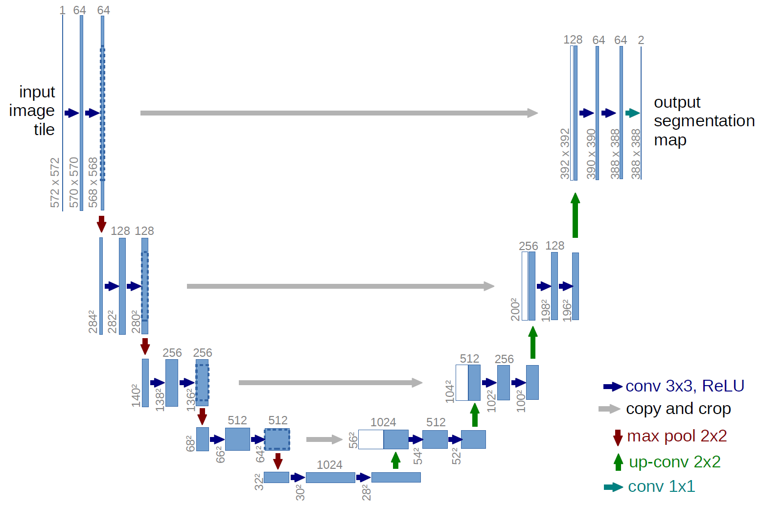
U-Net model architecture (image size at the output is smaller than the size of the input image; this is due to the fact that the network predicts worse at the edges of the image)

The author of U-Net has developed an architecture based on a different model - Fully convolutional network (FCN), a feature of which is the presence of only convolutional words (not counting max-pooling).
U-Net differs from FCN in that layers are added in which max-pooling is replaced with up-convolution. Thus, the new layers gradually increase the output resolution. Also, signs from the encoder part are combined with features from the decoder part, so that the model can make more accurate predictions with additional information.

A model in which there is no forwarding of signs from the encoder-part to the decoder-part is called SegNet and in practice shows results worse than U-Net.


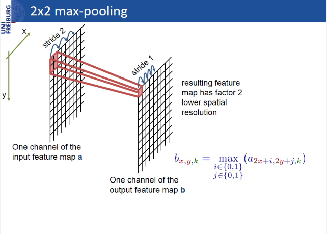
Max-pooling


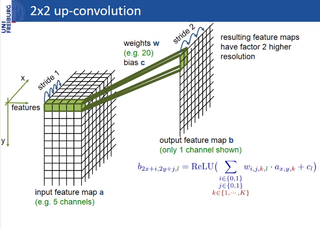
Up-convolution

The absence of layers attached to the image size in U-Net, Segnet and FCN allows to feed images of different sizes to the same network input (the image size must be a multiple of the number of filters in the first convolutional layer).

In keras, this is implemented as follows:

 inputs = Input((channel_number, None, None)) 

Learning, as well as prediction, can be conducted either on image fragments (crocs), or on the entire image as a whole, if GPU memory allows. In this case, in the first case:
1) more than the size of the batch, which will well affect the accuracy of the model, if the data is noisy and heterogeneous;
2) less risk of retraining, because There is much more data than when training on full-size images.

However, when learning on the crocks, the edge effect is more pronounced - the network predicts less accurately at the edges of the image than in areas closer to the center (the closer the prediction point to the border, the less information the network has on what is next). The problem can be solved by predicting a mask on fragments with overlaps and discarding or averaging the areas on the border.

U-Net is a simple and powerful architecture for a binary segmentation task, on github you can find more than one implementation for any DL framework, but for segmentation of a large number of classes, this architecture loses to other architectures, for example, PSP-Net. Here you can read an interesting review on architectures for semantic image segmentation.

Determining the height of buildings

The height of buildings can be determined by their shadows. To do this, you need to know: the size of the pixel in meters, the length of the shadow in pixels and the sun (solar) elevation angle (angle of the sun above the horizon).


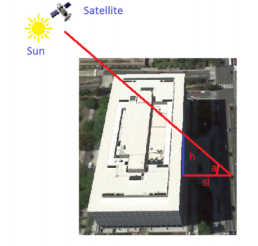
Geometry of the sun, satellite and building

The whole complexity of the task is to segment the building shadow as accurately as possible and determine the length of the shadow in pixels. Problems are also added by the presence of clouds in the pictures.

There are more accurate methods for determining the height of the building. For example, you can take into account the angle of the satellite above the horizon.



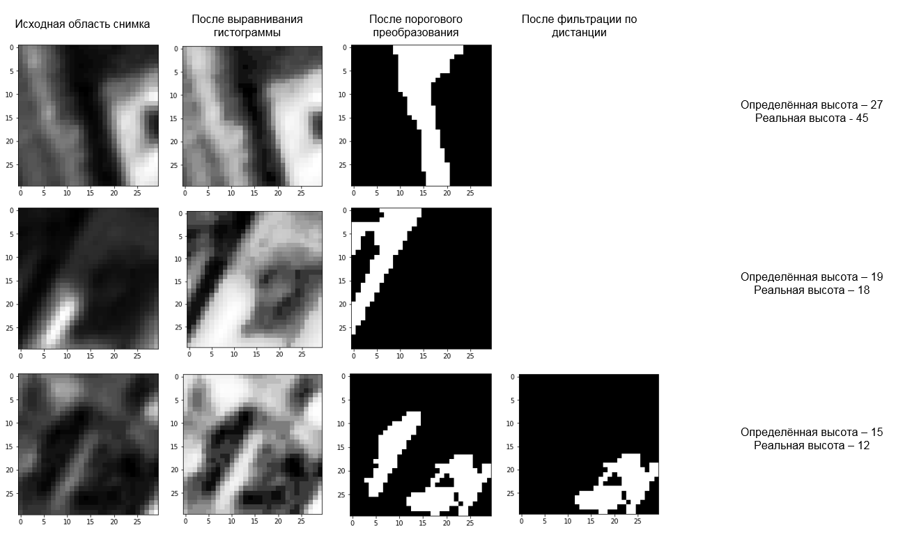
An example of the operation of the algorithm for determining the height of buildings by the shadow

In the images from the group of satellites PlanetScope with a spatial resolution of 3 m, the error in determining the height of buildings using the MAPE (mean absolute percentage error) was ~ 30%. A total of 40 buildings and one image were reviewed. However, in submeter shots, the researchers received an error of only 4-5% .

Conclusion

Remote sensing of the Earth provides many opportunities for analytics. For example, companies such as Orbital Insight, Spaceknow, Remote Sensing Metrics, OmniEarth and DataKind, on the basis of satellite imagery, monitor production and consumption in the United States, analyze urbanization, traffic, vegetation, the economy, etc. At the same time, the pictures themselves are becoming more accessible. For example, images from Landsat-8 and Sentinel-2 satellites with a spatial resolution of more than 10m are in the public domain and are constantly being updated.

In Russia, Sovzond, ScanEx, Racurs, Geo-Alliance and Northern Geographic Company also conduct geoanalytics using satellite images and are official distributors of satellite remote sensing operators: Russian Space Systems OJSC (Russia), DigitalGlobe (USA), Planet (USA ), Airbus Defense and Space (France-Germany), etc.

PS Yesterday we launched an online satellite imagery competition consisting of two tasks:

1. Segmentation of buildings and cars and car counting;
   
2. Determination of building heights.
   

So, anyone who is interested in the field of computer vision and remote sensing of the Earth, join!

We plan to hold another competition in the pictures of Roskosmos, Airbus Defense and Space and PlanetScope.