Optimization of securities portfolio using Python

Introduction

In the financial market, there are usually several types of securities: government securities, municipal bonds, corporate shares, etc.

If a market participant has free money, then they can be taken to a bank and receive interest or buy securities on them and receive additional income. But which bank to take? What securities to buy?

Low-risk securities tend to be low profitable, and high-yield securities tend to be more risky. Economic science can give some recommendations for resolving this issue, but for this it is necessary to have appropriate software, preferably with a simple interface and free.
')
Software for portfolio analysis should work with yield matrices and solve non-linear programming problems with constraints in the form of strict and non-strict inequalities. The symbolic solution in Python of some types of nonlinear programming problems I have already considered in the publication [1]. However, it is impossible to apply the methods proposed in this publication for the analysis of the securities portfolio due to limitations in the form of strict inequalities.

The purpose of this publication is to develop methods for optimizing securities portfolios using the scipy.optimize library. It was necessary to investigate and apply in programming such little-known possibilities of this library, as the introduction of additional restrictions to the objective function [2].

Statement of the problem of an optimal Markowitz portfolio

Consider the general task of allocating capital that a market participant wants to spend on acquiring securities. The goal of the investor is to invest money so as to preserve his capital, and, if possible, increase it.

A set of securities held by a market participant is called its portfolio. Portfolio value is the total value of all its constituent securities. If today its value is P, and in a year it will be equal to P, then it is natural to call (P'-P) / P yield of the portfolio in percent per annum. Portfolio returns are returns per unit of value.

Let xi be the share of capital spent on the purchase of securities of the i-th type. All allocated capital is taken as a unit. Let di be the yield in percent of the annual securities of the i-th type per one monetary unit.

Yield fluctuates over time, so we will consider it a random variable. Let mi , ri be the expected average return and the standard deviation, called risk. By CVij we denote the covariance of yields of securities of the i - and j - th types.

Every owner of a securities portfolio faces a dilemma: you want more efficiency and less risk. However, since “one cannot catch two birds with one stone”, it is necessary to make a certain choice between efficiency and risk.

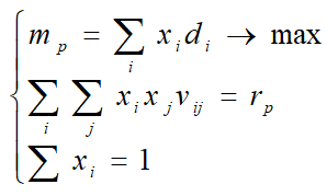
Markovits optimal portfolio model, which provides minimal risk and a given return

Such a model in the form of a system of equations and inequalities has the form [3]:



It is necessary to determine: x1, x2 ... xn.

The initial data for the calculation is the yield matrix of securities of the following form (filled example of the matrix in the program listing):



To implement the minimal risk model in Python, the following development steps must be performed:
1. Determination of average stock returns 1-6:

from sympy import * import numpy as np from scipy.optimize import minimize from sympy import * import numpy as np from scipy.optimize import minimize "D-   (   )" D=np.array([[9.889, 11.603,11.612, 12.721,11.453,12.102], [12.517, 13.25,12.947,12.596,12.853,13.036], [12.786, 12.822,15.447,14.452,15.143,16.247], [11.863, 12.114,13.359,13.437,11.913,15.300], [11.444, 13.292,13.703,11.504,13.406,15.255], [14.696, 15.946,16.829,17.698,16.051,17.140]],np.float64) d= np.zeros([6,1])#     m,n= D.shape#  for j in np.arange(0,n): for i in np.arange(0,m): d[j,0]=d[j,0]+D[i,j] d=d/n print("   1-6 : \n %s"%d) 

We get:

Average stock returns 1-6:

[[12.19916667]
[13.17116667]
[13.98283333]
[13.73466667]
[13.46983333]
[14.84666667]]

2. Construction of the covariance matrix (m = n = 6).

CV = np.zeros ([m, n])
for i in np.arange (0, m):
for j in np.arange (0, n):
x = np.array (D [0: m, j]). T
y = np.array (D [0: m, i]). T
X = np.vstack ((x, y))
CV [i, j] = round (np.cov (x, y, ddof = 0) [1,0], 3)
print (“Covariance matrix CV: \ n% s”% CV)

We get:

CV covariance matrix:

[[2.117 1.773 2.256 2.347 2.077 1.975]
[1.773 1.903 1.941 2.049 1.888 1.601]
[2.256 1.941 2.901 2.787 2.701 2.761]
[2.347 2.049 2.787 3.935 2.464 2.315]
[2.077 1.888 2.701 2.464 2.723 2.364]
[1.975 1.601 2.761 2.315 2.364 3.067]]

3. Symbolic definition of the function to determine the variance of the portfolio yield (risk function).

 x1,x2,x3,x4,x5,x6,x7,x8,p,q,w=symbols(' x1 x2 x3 x4 x5 x6 x7 x8 pqw' , float= True) v1=Matrix([x1,x2,x3,x4,x5,x6]) v2=v1.T w=0 for i in np.arange(0,m): for j in np.arange(0,n): w=w+v1[p.subs({p:i}),q.subs({q:0})]*v2[p.subs({p:0}),q.subs({q:j})]*CV[p.subs({p:i}),q.subs({q:j})] print("   ( ):\n%s"%w) 

We get:

Portfolio return variance (risk function):

2.117 * x1 ** 2 + 3.546 * x1 * x2 + 4.512 * x1 * x3 + 4.694 * x1 * x4 + 4.154 * x1 * x5 + 3.95 * x1 * x6 + 1.903 * x2 ** 2 + 3.882 * x2 * x3 + 4.098 * x2 * x4 + 3.776 * x2 * x5 + 3.202 * x2 * x6 + 2.901 * x3 ** 2 + 5.574 * x3 * x4 + 5.402 * x3 * x5 + 5.522 * x3 * x6 + 3.935 * x4 ** 2 + 4.928 * x4 * x5 + 4.63 * x4 * x6 + 2.723 * x5 ** 2 + 4.728 * x5 * x6 + 3.067 * x6 ** 2

4. Determining the optimal stock portfolio for minimum risk and return mp = 13.25

 def objective(x):#  x1=x[0];x2=x[1];x3=x[2]; x4=x[3]; x5=x[4]; x6=x[5] return 2.117*x1**2 + 3.546*x1*x2 + 4.512*x1*x3 + 4.694*x1*x4 + 4.154*x1*x5 + 3.95*x1*x6\ + 1.903*x2**2 + 3.882*x2*x3 + 4.098*x2*x4 + 3.776*x2*x5 + 3.202*x2*x6 + 2.901*x3**2 \ + 5.574*x3*x4 + 5.402*x3*x5 + 5.522*x3*x6 + 3.935*x4**2 + 4.928*x4*x5 + 4.63*x4*x6 \ + 2.723*x5**2 + 4.728*x5*x6 + 3.067*x6**2 def constraint1(x):#    -1 return x[0]+x[1]+x[2]+x[3]+x[4]+x[5]-1.0 def constraint2(x): #   return d[0,0]*x[0] + d[1,0]*x[1] + d[2,0]*x[2] + d[3,0]*x[3] + d[4,0]*x[4]+ d[5,0]*x[5] - 13.25 x0=[1,1,0,0,0,1]#        b=(0.0,1.0)#   x       bnds=(b,b,b,b,b,b)#    () con1={'type':'ineq','fun':constraint1} #    () con2={'type':'eq','fun':constraint2} #    () cons=[con1,con2]#    () sol=minimize(objective,x0,method='SLSQP',\ bounds=bnds,constraints=cons)#     print("   -%s"%str(round(sol.fun,3))) print(" 1 - %s, - %s"%(round(sol.x[0],3),round(d[0,0]*sol.x[0],3))) print(" 2 - %s, - %s"%(round(sol.x[1],3),round(d[1,0]*sol.x[1],3))) print(" 3 - %s, - %s"%(round(sol.x[2],3),round(d[2,0]*sol.x[2],3))) print(" 4 - %s, - %s"%(round(sol.x[3],3),round(d[3,0]*sol.x[3],3))) print(" 5 - %s, - %s"%(round(sol.x[4],3),round(d[4,0]*sol.x[4],3))) print(" 6 - %s, - %s"%(round(sol.x[5],3),round(d[5,0]*sol.x[5],3))) 

We get:

Minimum risk function -1.846
Share 1 share- 0.141, yield- 1.721
Share 2 share- 0.73, yield- 9.616
Share 3 share- 0.0, profitability- 0.0
Share 4 share- 0.0, yield- 0.0
Share 5 share- 0.0, profitability- 0.0
Share 6 share- 0.129, yield- 1.914

Conclusion:

Profitable are 1,2,6 shares. This is part of the answer to the questions posed at the beginning of the publication.

The optimal Markowitz portfolio of maximum return and given, (acceptable) risk

The system of equations and inequalities is:




Part of the listing does not require explanation, since everything is described in detail in the previous example. However, there are differences. The average yield column d and the condition function def constraint2 (x) are taken from the previous example, and in the previous example it was a minimum risk function. In addition, to determine the maximum, before defining the value of a new objective function — def objective (x), a minus sign is set.

Result:

Maximum yield function --14.1
Share 1 share- 0.0, yield- 0.0
Share 2 share- 0.72, yield- 9.489
Share 3 share- 0.0, profitability- 0.0
Share 4 share- 0.0, yield- 0.0
Share 5 share- 0.0, profitability- 0.0
Share 6 share- 0.311, yield- 4.611

Shares 2.6 are profitable. But this is not the only result of optimization with scipy optimize minimize minimize. I decided to compare the results with the solution of the same problem using Mathcad tools and this is what I got:



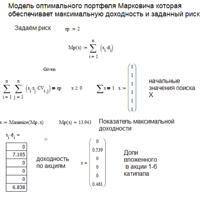
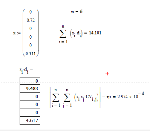
Mathcad points to the same numbers 2.6 profitable shares, but the shares are different. In Python 0.720,0.311 in Mathcad 0.539, 0.461, with different values ​​of the maximum yield, respectively, 14.1 and 13.9. In order to finally make sure which program calculates the optimum correctly, we substitute the values ​​of shares obtained in Python in Mathcad, we get:



Conclusion: Python has an optimum function, and therefore shares and profitability is calculated more accurately than when using Mathcad.

Formation of an optimal securities portfolio using the Tobin model

Tobin's Minimum Risk Portfolio:



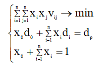
where d0 is efficiency without risky papers;
x0 is the share of capital invested in risk-free securities;
xi, xj - the share of capital invested in the securities of the i-th and j-th types;
di is the mathematical expectation (arithmetic average) of the yield of the i-th security;
vij is the correlation moment between the efficiency of the papers of the ith and jth species.

We select the share of capital of a given return, set the total yield, taking for example the following numerical values ​​x0 = 0.3, d0 = 10, dp = 12.7.


We get:

Minimum risk function: 0.728
Share 1 share- -0.023, yield: -0.286
Share 2 share- 0.666, yield: 8.778
Share 3 share- -1.0, yield: -13.983
Share 4 share- 0.079, yield: 1.089
Share 5 share- 0.3, yield: 4.048
Share 6 share- 0.677, yield: 10.054

Profitable shares are 2,4,5,6.

Tobin's portfolio of maximum efficiency

where rp is the portfolio risk.


We get:

Maximum profitability function: -11.657
Share 1 share- 0.09, yield: 1.096
Share 2 share- 0.196, yield: 2.583
Share 3 share- -1.0, yield: -13.983
Share 4 share- 0.113, yield: 1.552
Share 5 share- 0.411, yield: 5.538
Share 6 share- 0.463, yield 6.872

Profitable shares are 1,2,4,5.

Findings:

For the first time, Python solved the problem of optimizing a securities portfolio using Markowitz and Tobin models.
The comparative example with the Mathcad math package shows the benefits of the scipy optimize minimize minimize library.

References:

1. Character solution of nonlinear programming problems
2. scipy.optimize.minimize
3. Statement of the optimal portfolio problem