Automata programming. Part 4. Efficiency of auto-designed programs
I would put the question differently: how effective are auto-designed programs? Such a formulation of the question suggests that automaton design is a source of high program efficiency. I have hardly ever touched on such an important topic as efficiency , and the Display example is ideally suited to illustrate the efficiency of automated design. In the first article I introduced readers to the “laboratory” version of this module, but I will test the “combat” version, the design process of which I will give in the next article. A performance study will be performed for the msp430 and CortexM3 platforms.
In order not to be subjective, evaluating the effectiveness, it is necessary to compare the results with something. Therefore, I will conduct the same set of tests for the non-automatic implementation of the Display example, kindly provided by michael_vostrikov , for which he is very grateful and has his karma.
Automaton implementation, I conditionally call A1, non-automaton - A2. The original A2 is written in JavaScript, but in order to be able to explore these implementations on an equal footing, I perekatal version A2 in C ++ . From him and begin.
(FSM ||! FSM)?
As in the case with the implementation of A1, option A2 is divided into: a module for splitting text into blocks and a module for displaying text blocks.
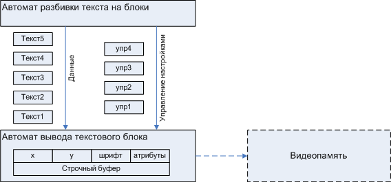
Figure 1. The large-scale structure of the module "A2 :: Display"
The blocking machine is represented by the function A2 :: tDisplay :: Out_text. From her analysis, it can be seen that option A2, conventionally called by me “non-automatic”, is implemented by a typical automaton, which is described by a state diagram:
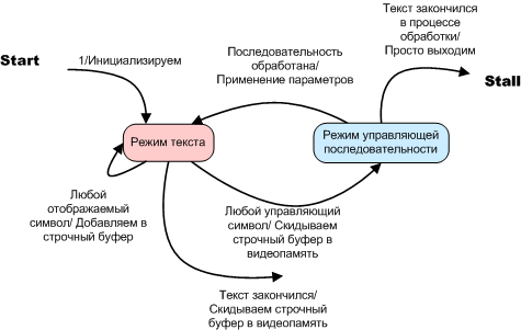
Figure 2. Option A2. Automatic text breaks into blocks. State diagram
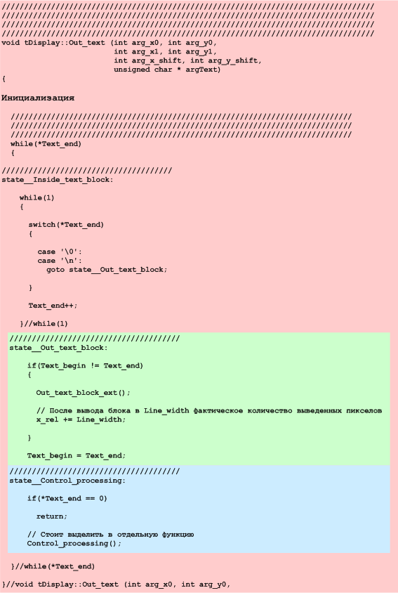
In order to emphasize the state in the source, I will highlight them in color.
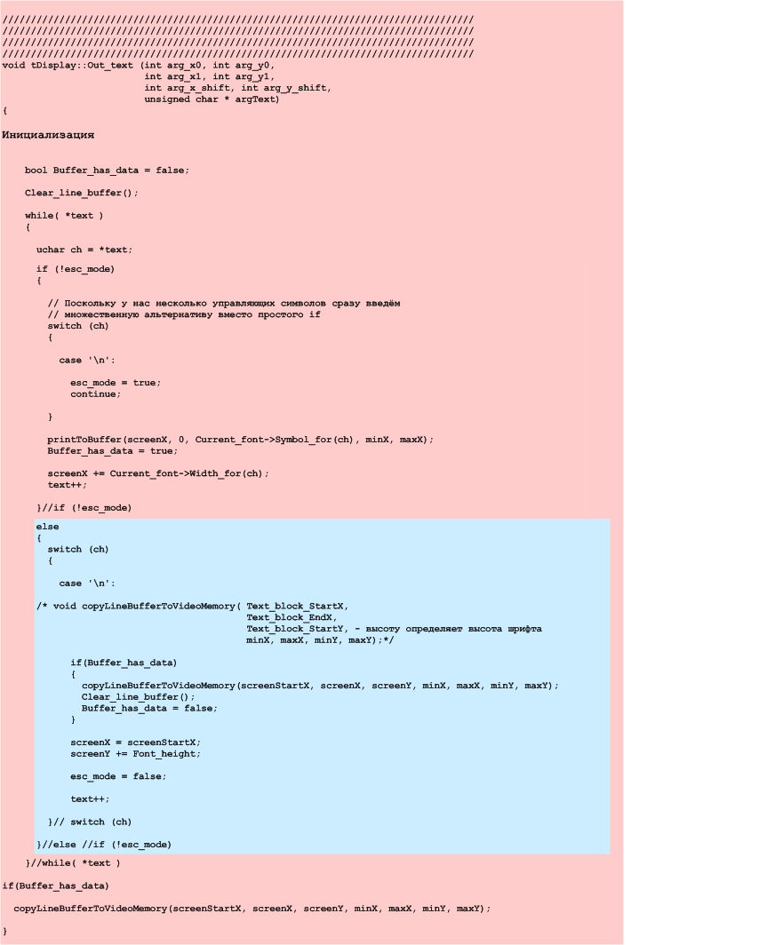
Figure 3. Option A2. Automatic text breaks into blocks. Source code of the program with “highlighted” states
The A2 automat :: tDisplay :: Out_text is another example of the implementation of automata after examples from the previous article. There are two explicitly selected states and a variable (esc_mode) that defines the current Internal state . The fact that this variable is of type bool does not detract from it in this capacity.
Consider a similar machine for option A1, which I give here for convenience
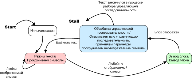
Figure 4. Option A1. Automatic text breaks into blocks. State diagram
It is also an automaton, it has three uniquely identified states and transitions between them are clearly spelled out, and although there is no special variable describing the internal state, the program structure is such that the program counter is this variable. When:
Table 1. Correspondence between the value of the program counter and the current internal state of the program
value of software counter in range | it corresponds to the state | |
state__inside_text_block | state__out_text_block | text mode |
state__out_text_block | state__control_processing | block output |
state __ control _ processing | until the end of the cycle | manager processing sequences |
In the case of A2, the variable type bool acts as a variable of the Internal state , in the case of A1, a program counter, and nevertheless these are pronounced automaton-implemented algorithms. Let me remind you that the option A2 is an automatic machine Miles. Unlike Moore’s automaton (variant A1), the output signals (or actions) are written here not in an oval, but above the transition arrow, through a slash after the transition condition.
A2 :: OA.
We continue the analysis of the option A2 :: Display, going to the automatic output of the text block. This machine is very different from the similar machine version A1.
struct tFont_item{ u1x Width; const u1x * Image; }; union { u2x Data; u1x Array[2]; }Symbol_buffer; //////////////////////////////////////////////////////////////////////////////////////// //////////////////////////////////////////////////////////////////////////////////////// //////////////////////////////////////////////////////////////////////////////////////// void printToBuffer( int lineStartX, int lineStartY, const tFont_item * symbolInfo, int minX, int maxX) { u1x bytes_Width = (symbolInfo->Width + 7) >> 3; for (int y = 0; y < Font_height; y++) { if(bytes_Width == 1) Symbol_buffer.Array[1] = *((u1x*)(symbolInfo->Image + bytes_Width * y)); else Symbol_buffer.Data = *((u2x*)(symbolInfo->Image + bytes_Width * y)); u2x bit_mask = 0x8000; for (int x = 0; x < symbolInfo->Width; x++) { bool bit = Symbol_buffer.Data & bit_mask; bit_mask = bit_mask >> 1; int lineX = lineStartX + x; int lineY = lineStartY + y; if (lineX >= minX && lineX <= maxX) { setPixelInBuffer(lineX, lineY, bit); } }//for (int x = 0; x < symbolInfo->Width; x++) }//for (int y = 0; y < Font_height; y++) };//void printToBuffer( int lineStartX, int lineStartY, tFont_item * symbolInfo, int minX, int maxX ) //////////////////////////////////////////////////////////////////////////////////////// //////////////////////////////////////////////////////////////////////////////////////// //////////////////////////////////////////////////////////////////////////////////////// void setPixelInBuffer(int x, int y, bool bit) { int bitNumber = (x & 7); int byteNumber = x >> 3; if (bit) { Line_buffer[y][byteNumber] |= (0x80 >> bitNumber); } };//void setPixelInBuffer(int x, int y, bool bit) In this implementation, no classification of symbols is performed, therefore, the operation of the UA for the Automat of outputting a text block is reduced to a direct call to the operational automaton for displaying the symbol for each displayed symbol.
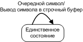
Figure 5. Text block output machine, control machine
But where does the automatic machine come from in a non-automatic implementation? Despite the fact that the implementation of the A2 was conditionally called non-automatic, it is also based on an operating machine. This is the simplest arbitrary bitwise automaton.
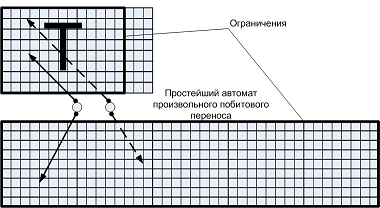
Figure 6. Example A2 operation machine
As mentioned earlier, the operating machine is a semi-finished product that can perform some action with any valid parameters. It may be degenerate into a combinational circuit. The main requirements for it: maximum simplicity, maximum efficiency. These requirements, as will be shown, are in conflict.
From the point of view of the simplicity of the algorithm, the operating machine of an arbitrary bit-wise transfer is excellent. It is universal; it can copy any pixel of a character generator into an arbitrary pixel of a line buffer. Parameterization of OA in this case is carried out by the simplest control automaton.

Figure 7. Control Output Machine
This example shows that the majority of programs with simple control logic are auto-implemented by themselves, the manuality appears when a sequential complication of the control logic occurs. If you do not design the algorithm as an explicit automaton, then with the sequential complication of the program, after adding another chip, another “crutch”, a “structural transition” can occur - the automatic implementation will disappear and you will get something like the non-automatic example from articles 2 and 3.
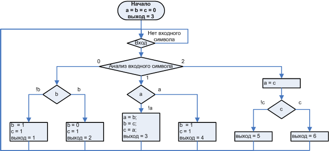
Figure 8. Non-automatic algorithm
So, we had the opportunity to make sure that the implementation of A2 in its pure form is automatic, but how effective is it?
A1 vs A2
The only way to compare the effectiveness of the implementations in question is to conduct tests. For testing, I use the IAR development environment .
The first test example - a string of characters in full screen, displayed in the form of a line running from right to left, until the entire line disappears from the screen. The physical output is emulated by data output to the I / O port, which corresponds to reality in the first approximation.
Font 6x9, display 256x64. Optimization - maximum speed.
char Test_text[43]; int main( void ) { for(int i = 0; i < 42; i++) Test_text[i] = 'A' + i; Display = new tDisplay(256,64,16); for( int i = 0; i > -270 ; i-- ) { Display->Out_text(0,0,256,64,i,0, (uchar*)Test_text); } } To do this, right in the IAR editor, I created a file and saved it as cspy_1.mac . In the file put the text with macrofunctions
__var filehandle; //////////////////////////////////////////////// setup() { filehandle = __openFile("filelog1.txt", "w"); } //////////////////////////////////////////////// clear() { #CCTIMER1 = 0; } //////////////////////////////////////////////// out_data() { __fmessage filehandle , #CCTIMER1, "\n"; #CCTIMER1 = 0; } //////////////////////////////////////////////// close() { __closeFile(filehandle); } This C is a similar language, but not C, is very simple and is described in some detail in the IAR help. Then I connected this file to the project. For this, I selected the Debugger item via Project-> Options , checked the Use macro file checkbox and selected the file cspy_1.mac .
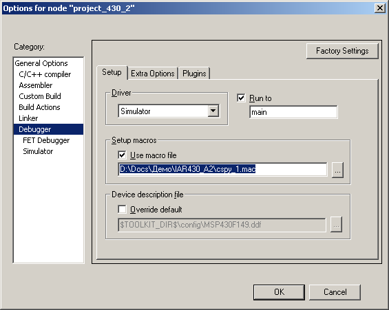
Figure sp.1. Connecting to the project file with macrofunctions
The macro functions described in cspy_1.mac are connected to the breakpoints shown in Fig. sp.2.
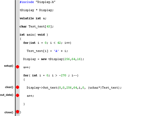
Figure sp.2. Connect breakpoints
To this end, breakpoints are placed in the positions of interest. Breakpoints are set and removed by double clicking on the gray bar to the left of the text. After all the points are set, you need to open the View-> Breakpoints tab
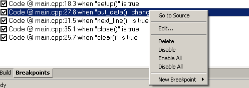
Figure sp.3. Customization
Right-click on the point of interest, select Edit, the Edit breakpoint window appears.
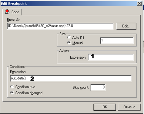
Figure sp.4. Customization
In the window that appears, the name of the required function is written. If you register it in the field labeled 1, then the specified function will be called only when a stop occurs. In order for the specified function to be called, but without stopping the program, its name should be entered in field 2, which will cause this function to be called until it stops, in order to determine whether the program should be stopped or not. If the corresponding macro function returns 1, it will stop if the function returns 0 or returns nothing, there will be no stop. The specified macro function will be executed before the execution of the corresponding C program expression at the breakpoint.
The results of the study are shown in the graph.
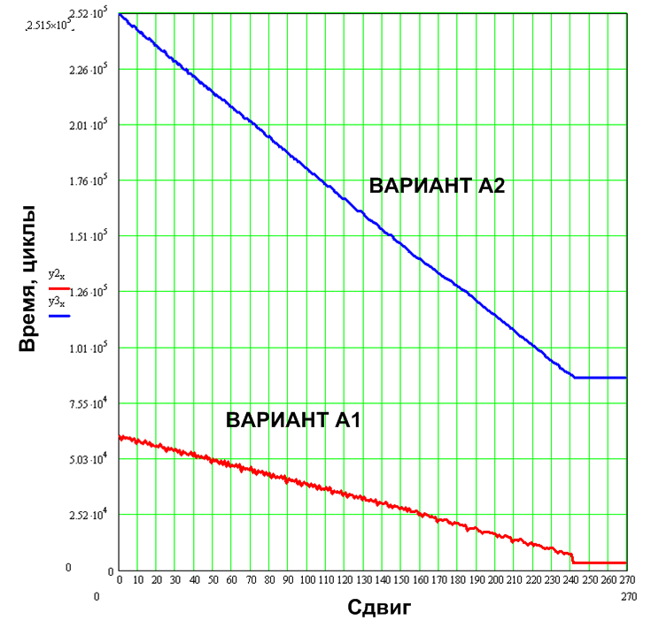
Figure 9. Results of the first test
It is well seen that for option A2, when the line actually goes beyond the edge of the output window, a significant number of cycles are spent so that, as a result, nothing is shown. A verification option is possible, but it will slow down the algorithm even more if there is something to output. For variant A1, when the line goes out of the window, the cyclic consumption drops to around 3000 cycles. This behavior is initially built into the structure of the algorithm itself by selecting the appropriate states of the automaton (in the next article I will describe the automata process using the example of A1), it does not require additional checks.
The first example gives a general idea of how these two algorithms work in the running line mode, but the main use of the Display module is the usual output of text that fits completely on the screen to any position on the screen. To study the operation of the module in the main mode, I will use the test example:
char Test_text[32]; int main( void ) { for(int i = 0; i< 31; i++) Test_text[i] = 'A' + i; Display = new tDisplay(256,64,24); for( int j = 0; j < 31; j++) { for( int i = 0; i < 8; i++) { Display->Out_text(0,0,256,64,i,0, (uchar*)&Test_text[31-j]); } } } The test example displays lines of different lengths from 0 to 31 characters, 6x9 font. Each line is displayed first without a shift, then with a shift of 1 pixel to the right, then by 2, and so on. up to 8 pixels. This simulates text output, in different positions of the screen (to which both algorithms are sensitive).
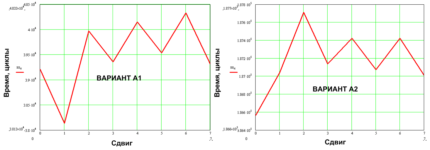
Figure 10. The effect of the initial shift of the output window from the byte boundary to cyclic consumption
The results obtained are averaged by the shifts, the result is a value that does not depend on the initial position of the line on the screen.
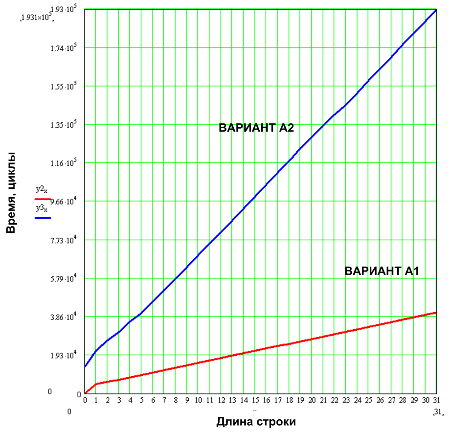
Figure 11. Displaying a text string in 6x9 font
As one would expect, the value of cyclic consumption grows linearly with an increase in the number of characters in a line. For variant A1, the specific cycle consumption (cycles per symbol) is 1200 cycles per symbol, for variant A2 5913 cycles (optimization, I remind, the maximum in speed).
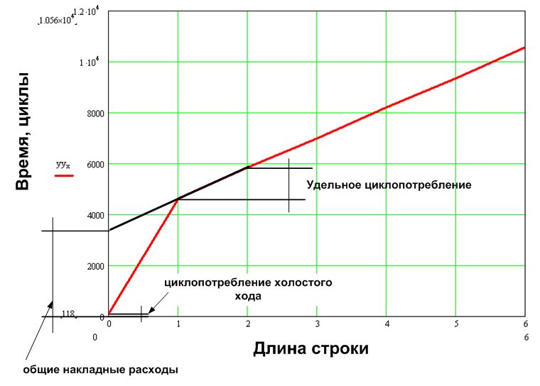
Figure 12. Explanation of terms: total overhead, specific cycle consumption, and cycle consumption of idle
Total overheads are 3431 (A1) and 16433 (A2). It is worth paying attention to the cyclic consumption of idling , that is, when the input is a string with a length of 0 characters - 118 (A1) and 13548 (A2) cycles. Such a gigantic difference is connected with the cleaning of the line buffer in the A2 variant. Using an additional check of the source line to the '\ 0' character, you can eliminate the cleaning of the string buffer for the empty line and reduce the cyclic consumption of idle to a value comparable to A1. I did not do it intentionally, in order to have a good reason to consider in more detail the question of the lower-case buffer. Work with the line buffer is the main component of the large overhead. First, it is possible to exclude the operation of cleaning the string buffer, if we rewrite the setPixelInBuffer function
void setPixelInBuffer(int x, int y, bool bit) { int bitNumber = (x & 7); int byteNumber = x >> 3; if (bit) { Line_buffer[y][byteNumber] |= (0x80 >> bitNumber); } else { Line_buffer[y][byteNumber] &= ~(0x80 >> bitNumber); } };//void setPixelInBuffer(int x, int y, bool bit) but in this case, not acceleration is obtained, but the algorithm slows down about 1.5 times (for a 6x9 font) per character, because when cleaning the line buffer, all “white” pixels are output at once, and in this variant each “white” pixel is displayed separately. Graph Fig. show the picture that will turn out in this case.
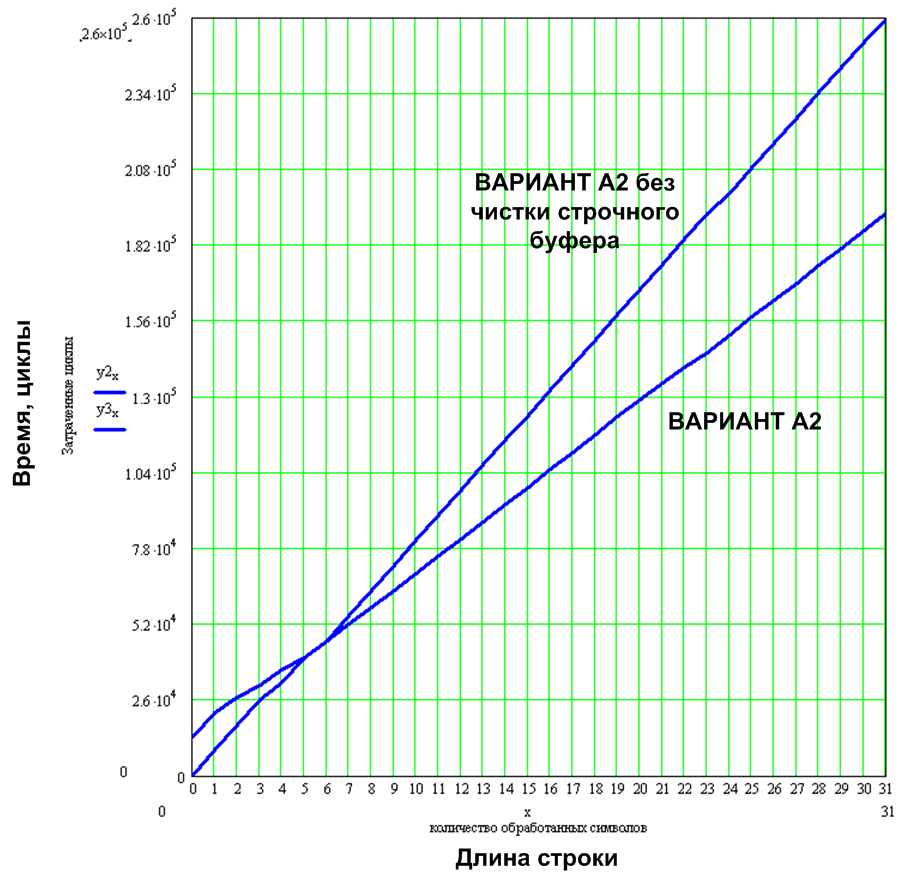
Figure 13. Difference between implementations with and without line buffer cleaning
The second problem related to the line buffer is not connected with the need to clean the line buffer, but in its very presence. For a display of 256 pixels wide and maximum font height of 24 pixels, the size of the line buffer is 768 bytes. For “small” microcontrollers in general and msp430 in particular, the problem of RAM deficiency is typical. The line buffer option requires:
This turns out to be very wasteful for microcontrollers with a RAM size of 2-4 kb. And this is despite the fact that the same controller contains a 60 kb ROM and the program code of the tDisplay module occupies the same 2 kb of the code - 3.2%. 3.2% for the basic I / O function (which already contains an efficient implementation of the crawl and virtual output windows) is very acceptable, while 41.5% of the RAM for one text output operation is a serious expense. Even if you take a more solid msp430f2616 with 4 KB of RAM, then 20% is still not small.
If we are talking about msp, it would not be superfluous to say about energy saving. This is one of the most modest power supply microcontrollers, which is well suited to work in devices powered by batteries. I draw attention to perhaps not the most obvious aspect: a multiple increase in program speed not only speeds up the work as a whole (speed is not always critical), but directly saves battery energy , allowing the microcontroller to sleep for most of the time, and one charge multiple times.
Option A1 is designed according to the scheme without line buffer. That is, this module is not only many times faster, but also requires ten times less RAM. The automatic machine used in A1 has two sub-realizations: speed and economical. Economical requires to work only about 60 bytes of RAM. The question naturally arises: is it likely that variant A1 loses to variant A2 in the amount of code? Indeed, with full optimization in speed (at which, however, some optimization in size is made), we obtain the following picture in terms of characteristics.
Table 2. Comparative characteristics of software modules
pzu | ram | performance | |
a2 | 1122 | 796 + 58 stack | one |
a1. speed | 2088 | 240 + 26 stack | 4.6 - 7.9 |
a1.economic | 2490 | 62 + 18 stack | 3.5 - 6 |
For comparison, the size of the character generator for which the glyphs of all 256 characters are defined, for a 6x9 font is 3344 bytes.
Let us analyze how the specific cycle consumption grows with increasing font size. In fig. 14 shows a graph of the specific cyclic consumption for the 6x9, 8x16 and 16x24 fonts, which shows that the value of the AC for variant A2 is proportional to the area, and for variant A1 it is proportional to the height of the characters. To emphasize this, the x-axis shows the area of symbols for the A2 variant, and for A1 the height of the symbol in the lines.
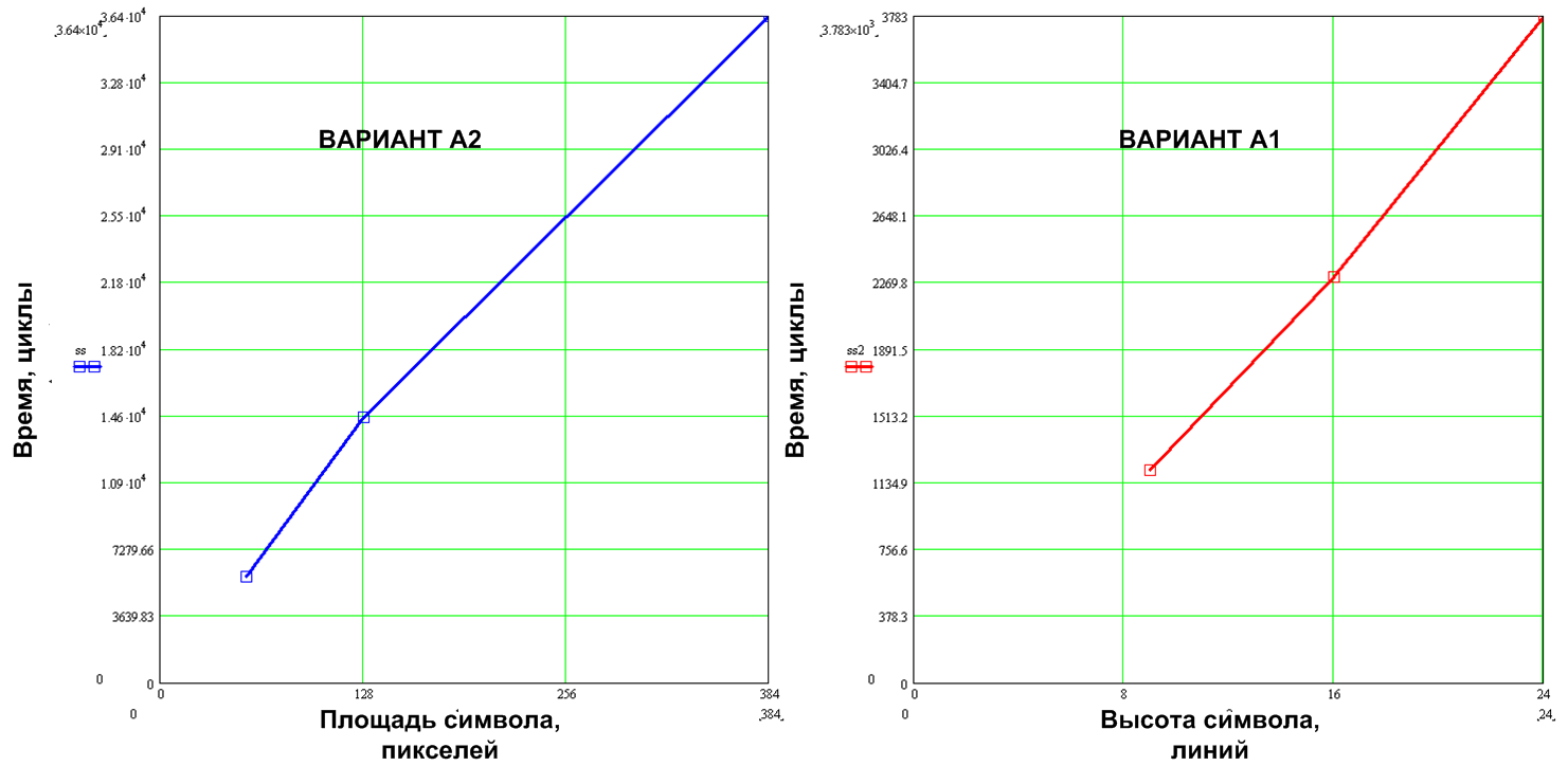
Figure 14. The dependence of the specific cyclic consumption of the font size
Specific cycloconsumption of variant A1 (hereinafter all the figures for speed), compared with A2, is higher by 4.9 for the 6x9 font, 6.4 times for the 8x16 font and 9.2 times for 16x24, and on average, for the line with length 0..31, the A1 variant shows more The speed is 4.6 times for the 6x9 font, 5.8 times for 8x16 and 7.9 times for 16x24.
A look into the future.
Let me propose for consideration an important issue that goes far beyond the scope of this series of articles. The test modules had maximum speed optimization. I would like to know how these implementations optimize. In fig. 15 shows the optimization coefficient (the ratio of non-optimized to optimized) depending on the length of the string, for different fonts, for both options.
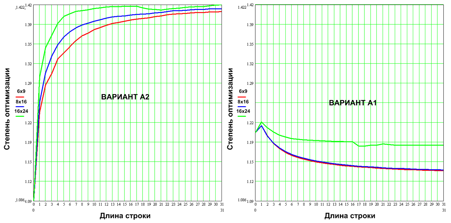
Figure 15. The degree of optimization of the program
It can be seen that the degree of “compression” in both variants is small, which means that we are not talking about good and bad implementation, both options are implemented effectively for their scheme , i.e. OA + UA But note that even the option A2 compressed by 1.4 times is 5-8 times slower than the compressed total 1.15 times of variant A1. And this is not surprising, the main tools of the optimizer are: inline function insertion, loop optimization, unfolding of short loops and so on. Those. It optimizes standard programming programming structures. But the optimization of the algorithm, like the optimization of the automaton (Fig. 16) underlying the program, gives a significant performance boost, and this is the leitmotif of today's article.
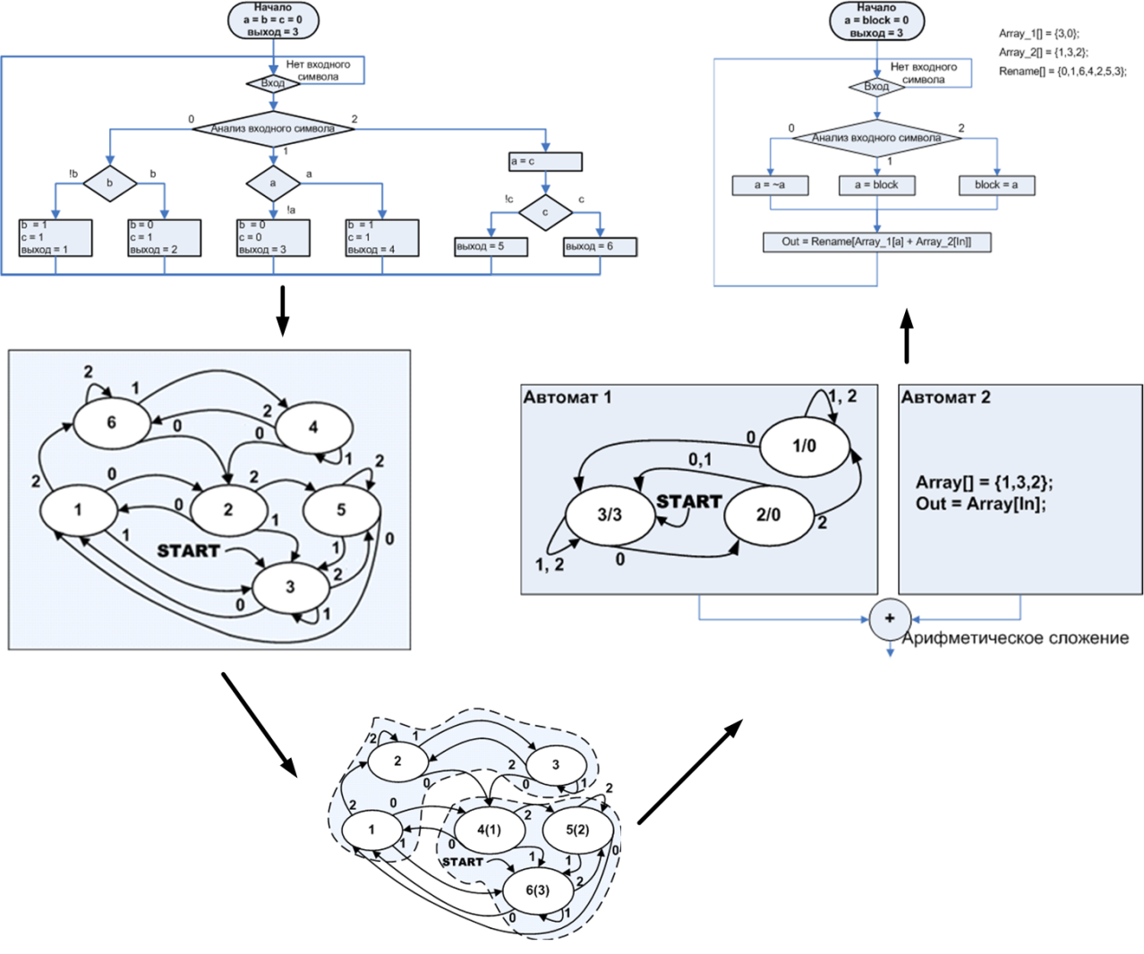
Figure 16. Optimization of the algorithm by optimizing the corresponding automata
From here you can make a far-reaching conclusion: one of the ways of the evolution of code optimizers is associated with the transformation of the algorithm into an automaton, and the optimization of the resulting automaton. However, in the example of the A2, such primitive automata are such that there is no place to optimize them further. 1 2 . , 2, 1, 2. «» , , :
1. . , . , , , , . , - . , , , .

17.
, (, , IAR visualState), , , 1 , 2 .
2. , , . Those. , . , « » , , «» , .
18.
3. , . .

19.
( , ).
, . (VHDL), , , ( ), , -, , . , , .
, , , . , , . , .
(.. ) , – , . , ( ), .
, . , , . , — ( ), , .
20.
. , .
, . . , . , , , . , , . , , CortexM3
CortexM3
, . msp 430.
3.
69 | 816 | 1624 | ||||
msp430.a1 | 3431 | 1202 | 6122 | 2299 | 7764 | 4052 |
msp430.a2 | 15938 | 5716 | 28910 | 14318 | 42402 | 35748 |
cortex m3.a1 | 1831(1.9) | 715(1.7) | 3237(1.9) | 1370 (1.7) | 4795(1.6) | 2238(1.8) |
cortex m 3. a 2 | 6182(2.6) | 2131(2.7) | 11347 (2.5) | 5236(2.7) | 16440(2.6) | 13282(2.7) |
. Cortex M3. 1-2 , msp430 ( -) 2-3 . – . Cortex M3 32 32 , , msp430 16 1 .
msp430: 1043 1122 2 1914 2088 1.. 200 , 1. .
– . — . 1 , .
Source: https://habr.com/ru/post/341888/
All Articles