Selected chapters of the control theory on fingers: linear observers of dynamic systems
I continue to write about the theory of management "on the fingers." To understand the current text, it is necessary to read the two previous articles:
I am not at all an expert in management theory, I only read textbooks. My task is to understand the theory and put it into practice. In this article, only the theory (well, a little accompanying code), next we will talk about the practice, a small piece of which can be found here:
Corrections and additions are welcome. For the hundredth time I remind you that first of all I write these texts for myself, as it forces me to structure knowledge in my head. This site is for me a kind of public address book, to which, by the way, I myself regularly return. Just in case, let me remind a bearded joke that describes my life well:
')
So, let's recall what we talked about in the last article , namely, what the Russian school calls analytical design of optimal regulators. I will even take an example from that article.
Suppose we have a car whose state at a given time k is characterized by its x_k coordinate and v_k speed. The experiment begins with a certain initial state (x_0, v_0), and our task is to stop the car at zero coordinates. We can affect it through gas / brakes, that is, through acceleration u_k. We write this information in a form that is convenient to transfer from person to person, because The verbal description is cumbersome and can allow several tacings:
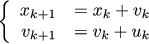
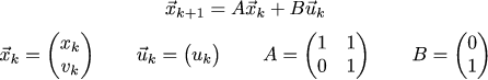
It is even more convenient to write this information in a matrix form, since the matrices can be substituted into this formulation by the most diverse, thus the language is very flexible and can describe many different problems:
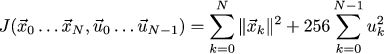
So, we described the dynamics of the system, but we did not describe either the goal, or what exactly is considered good governance. Let's write the following quadratic function, which takes as parameters the vehicle trajectory and the sequence of control signals:
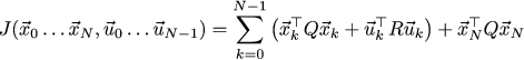
We try to find a vehicle trajectory that minimizes the value of this function. This function sets a compromise of goals: we want the system to converge to zero as quickly as possible, while maintaining a reasonable amount of control (no need to slow down the skid!)
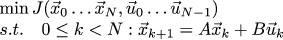
So we have the task of minimizing the function with a linear restriction on the input variables. For our specific problem about the car last time we chose such weights 1 and 256 for our purposes:
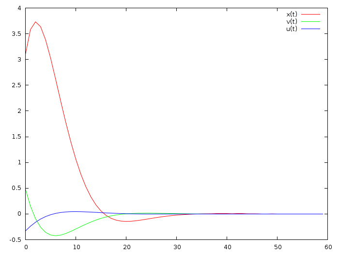
If at the initial moment our car is in position 3.1 and has a speed of half a meter per second, then the optimal control looks like this (I quote a picture from the previous article):
Let's try to draw the same curves in a slightly different way than last time. To write sums is very cumbersome, let's reduce to a matrix view. First of all, our entire trajectory and our entire control sequence are summarized into healthy matrix columns:
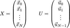
Then the relationship of the coordinates with the control can be written as follows:
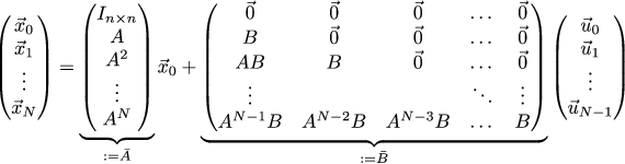
Or even more briefly:
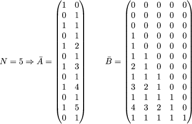
In this article, the sticks above the matrices mean the reduction of small matrices that describe one iteration into large ones for the whole task. For our particular problem, the powers of the matrix A ^ n are as follows:
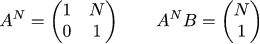
For clarity, let's explicitly write Ā and B̄:
And even give the source code that fills these matrices in numpy:
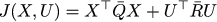
Let us summarize in large matrices and coefficients of our quadratic form:

In our specific problem about the car, Q̄ is the identity matrix, and R̄ is the identity multiplied by the scalar 256. Then the control quality function is written in matrix form very briefly:
And we are looking for the minimum of this function with one linear constraint:
Note to yourself: an excellent reason to deal with the Lagrange multipliers, the Legendre transform and the Hamiltonian function derived from this. And also how this explains the explanation of LQR through dynamic programming and the Riccati equations. Apparently, still need to write articles :)
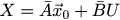
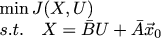
I'm lazy, so this time we will go the most direct way. J depends on two arguments that are linearly related to each other. Instead of minimizing the function with linear constraints, let's just remove the unnecessary variables from it, namely replace the occurrences of X with Ā x_0 + B̄ U in it:
This is quite tedious, but completely mechanical and does not require a brain output. In the transition from the penultimate line to the last, we took advantage of the fact that Q̄ is symmetric, it allowed us to write Q̄ + Q̄ ^ T = 2 Q̄.
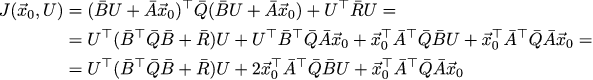
Now we just need to find the minimum of a quadratic function, no restrictions on variables are imposed. We recall the tenth grade of the school and equate to zero the partial derivatives.
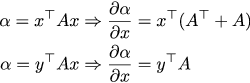
If you are able to differentiate ordinary polynomials, then you can take derivatives from matrix ones. Just in case, let me remind the rules of differentiation:
Again the smallest tedious writing of scribbles and we get our partial derivative with respect to the control vector U (we again used the symmetry of Q̄ and R̄):
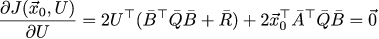
Then the optimal control vector U * can be found as follows:
Well, how do we write squiggles, but still have not drawn anything yet? Let's get better!
This will give the following picture, note that it perfectly coincides with the one that we received in the last article (drawing here ):
So, the theory tells us that (for a far horizon of events) the optimal control linearly depends on the remaining distance to the final goal. Last time we proved it for a one-dimensional case, in a two-dimensional case, having believed in the word. This time again I will not strictly prove, leaving it for a later conversation about Lagrange multipliers. However, it is intuitively clear that this is the case. After all, we have obtained the formula U = K * x0, where the matrix K does not depend on the state of the system, but only on the structure of the differential equation (on the matrices A and B).
That is, u_0 = k_0 * x_0. By the way, we got k_0 equal to [-0.052 -0.354]:
Compare this result with what I obtained with the help of the OLS and the one that was obtained by solving the Riccati equation (in the comments to the previous article). It is intuitively clear that if u0 depends linearly on x_0, then for a far horizon of events the same should be for x1.
Continuing the argument, we expect that the control u_i should be considered as u_i = k_0 * x_i. That is, the optimal control should be obtained by the scalar product of the constant vector k_0 and the residual distance to the target x_i.
But our result is exactly the opposite! We found that u_i = k_i * x_0! That is, we found the sequence k_i, which depends only on the structure of the system equation, but not on its state. And the control is obtained using the scalar product of a constant vector (the initial position of the system) and the sequence found ...
That is, if everything is good, then we should have the equality k_0 * x_i = u_i = k_i * x_0. Let's draw an illustrative graph, taking x_0 for simplicity equal to k_0. Along one axis of the graph we will postpone the coordinate of the machine, along the other the speed. Starting from one point k_0 = x_0 we get two different sequences of points k_i and x_i converging to zero coordinates.
Drawing is available here .
If roughly, then k_i * x_0 form a sequence of projections k_i onto the vector x_0. The same for k_0 * x_i, is a sequence of projections x_i on k_0. On our graph it is clearly seen that these projections coincide. Once again, this is not proof, but only an illustration.
Thus, we have obtained a dynamic system of the form x_ {k + 1} = (A + BK) x_k. If the eigenvalues of the matrix A + BK are less than unity in absolute value, then this system converges to the origin for any initial x_0. In other words, the solution of this differential equation is the (matrix) exponent.
As an illustration, I randomly selected several hundred different x_0, and drew the trajectories of our typewriter. Drawing to take here . Here is the resulting picture:
All trajectories safely converge to zero, a slight twisting of the trajectories suggests that the matrix A + BK is a rotation and contraction matrix (it has complex eigenvalues smaller than one in absolute value). If I'm not mistaken, then this picture is called a phase portrait.
So, we cheerfully minimized our function J, and obtained the optimal control vector U0 as K * X0:
Is there still a difference between considering management in the same way or as u_i = k_0 * x_i? There is a colossal, if we have unaccounted factors in the system (that is, almost always). Let's imagine that our car is not rolling on a horizontal surface, but such a slide can meet on its way:
If we calculate the optimal control without regard to this slide, then trouble can happen
(drawing here ):
The machine not only will not stop, but will go to infinity to the right altogether, I even drew a third of the x_i graphics, and then it grows linearly. If we close the control loop, then small disturbances in the dynamics of the system do not lead to catastrophic consequences:
So, we are able to manage a dynamic system so that it strives to get to the origin. But what if we wanted the car to stop not at x = 0, but at x = 3? Obviously, it is enough to subtract the desired result from the current state x_i, and then everything is as usual. Moreover, this desired result may well not be permanent, but change over time. Can we follow another dynamic system?
Let's assume that we do not control our typewriter directly, but at the same time we want to follow it. We measure both states of the machine with the help of some sensors that have a rather low resolution:
I just took our curves and blundered their values. Let's try to filter the noise introduced by the measurements. As usual, we arm ourselves with the smallest squares.
So, our machine obeys the law x_ {k + 1} = A x_k + B u_k, so let's build a diffur observer that follows the same law:
Here y_k is a corrective member, through which we will inform our observer how far we are from the real state of affairs. Like last time, we write the equation in matrix form:
Okay. Now what do we want? We want the correction terms y_k to be small, and that z_k converge to x_k:
Like last time, we express Z through Y, we equate the partial derivatives with respect to Y to zero, and we obtain the expression for the optimal corrective term:

Then vague forebodings begin to torment me ... I have already seen it somewhere! Well, let's remember how X is related to U, we get the following expression:

But this is accurate to renaming the letters for U *! And in fact, let's go back a little bit, we rushed into business too quickly. Combining the dynamics for x_k with the dynamics for z_k we get the dynamics for the error x_k-z_k.

That is, our task of tracking a typewriter is absolutely equivalent to the problem of a linear-quadratic controller. Find the optimal gain matrix, which in our case will be equal to [[-0.594, -0.673], [- 0.079, -0.774]], and we get the following observer code:
But the filtered curves, they are not ideal, but still closer to reality than measurements with low resolution.
The dynamics of the system is determined by the eigenvalues of the matrix [[1-0.594.1-0.673], [- 0.079.1-0.774]], which are equal (0.316 + - 0.133 i).
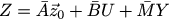
And let's go even further. Let's assume that we can measure only the position, but there is no sensor speed. Will we be able to build an observer in this case? Here we go beyond the LQR, but not too far. Let's write the following system:
Matrix C dictates to us what we can actually observe in our system. Our task is to find such a matrix L, which will allow the observer to behave well. Let's prescribe that the eigenvalues of the matrix A + LC, which describes the overall dynamics of the observer, should be about the same as the eigenvalues of the matrix from the previous example. Let's approximate the previous eigenvalues with fractions (1/3 + - 1/6 i). We write the characteristic polynomial of the matrix A + LC, and make it equal to the polynomial (x- (1/3 + 1/6 * i)) * (x- (1 / 3-1 / 6 * i). Then we solve the simplest system from linear equations, and the matrix L is found.


Calculations can be checked here , and drawing charts here .
This is how the work schedules of our observer look like, if we measure (and with a large error) only the coordinate of our machine:
From very incomplete data, we can very well restore the dynamics of the entire system! By the way, the linear observer that we built in fact is the famous Kalman filter, but we will talk about this some time next.
If, nevertheless, to bring to the logical end the computations of Y * (code is taken here) , then the final observer curves are much much smoother (and closer to the truth!) Than those that should be equivalent to them. Why?
- Least squares methods
- Linear-square controller, input
- Line square controller and linear observers
I am not at all an expert in management theory, I only read textbooks. My task is to understand the theory and put it into practice. In this article, only the theory (well, a little accompanying code), next we will talk about the practice, a small piece of which can be found here:
Corrections and additions are welcome. For the hundredth time I remind you that first of all I write these texts for myself, as it forces me to structure knowledge in my head. This site is for me a kind of public address book, to which, by the way, I myself regularly return. Just in case, let me remind a bearded joke that describes my life well:
')
A conversation between two teachers:
- Well, I got a group of stupid this year!
- Why?
- Imagine, explain the theorem - do not understand! Explaining a second time - do not understand! For the third time I explain, I already understood. But they do not understand ...
Linear-square regulator, side view
LQR: Problem statement
So, let's recall what we talked about in the last article , namely, what the Russian school calls analytical design of optimal regulators. I will even take an example from that article.
Suppose we have a car whose state at a given time k is characterized by its x_k coordinate and v_k speed. The experiment begins with a certain initial state (x_0, v_0), and our task is to stop the car at zero coordinates. We can affect it through gas / brakes, that is, through acceleration u_k. We write this information in a form that is convenient to transfer from person to person, because The verbal description is cumbersome and can allow several tacings:
It is even more convenient to write this information in a matrix form, since the matrices can be substituted into this formulation by the most diverse, thus the language is very flexible and can describe many different problems:
So, we described the dynamics of the system, but we did not describe either the goal, or what exactly is considered good governance. Let's write the following quadratic function, which takes as parameters the vehicle trajectory and the sequence of control signals:
We try to find a vehicle trajectory that minimizes the value of this function. This function sets a compromise of goals: we want the system to converge to zero as quickly as possible, while maintaining a reasonable amount of control (no need to slow down the skid!)
So we have the task of minimizing the function with a linear restriction on the input variables. For our specific problem about the car last time we chose such weights 1 and 256 for our purposes:
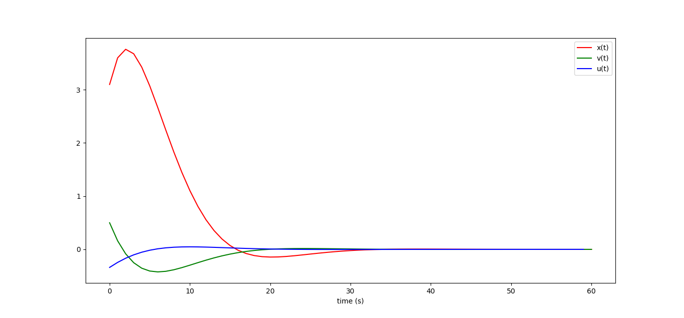
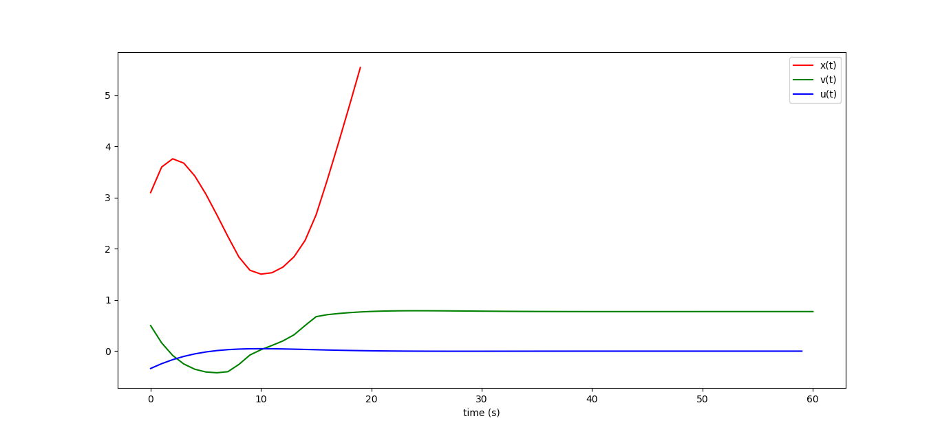
If at the initial moment our car is in position 3.1 and has a speed of half a meter per second, then the optimal control looks like this (I quote a picture from the previous article):
LQR: Solving the problem
Let's try to draw the same curves in a slightly different way than last time. To write sums is very cumbersome, let's reduce to a matrix view. First of all, our entire trajectory and our entire control sequence are summarized into healthy matrix columns:
Then the relationship of the coordinates with the control can be written as follows:
Or even more briefly:
In this article, the sticks above the matrices mean the reduction of small matrices that describe one iteration into large ones for the whole task. For our particular problem, the powers of the matrix A ^ n are as follows:
For clarity, let's explicitly write Ā and B̄:
And even give the source code that fills these matrices in numpy:
import matplotlib.pyplot as plt import numpy as np np.set_printoptions(precision=3,suppress=True,linewidth=128,threshold=100000) def build_Abar(A, N): n = A.shape[0] Abar = np.matrix( np.zeros(((N+1)*n,n)) ) for i in range(N+1): Abar[i*n:(i+1)*n,:] = A**i return Abar def build_Bbar(A, B, N): (n,m) = B.shape Bbar = np.matrix( np.zeros(((N+1)*n,N*m)) ) for i in range(N): for j in range(Ni): Bbar[(Ni)*n:(N-i+1)*n,(Nij-1)*m:(Nij)*m] = (A**j)*B return Bbar A = np.matrix([[1,1],[0,1]]) B = np.matrix([[0],[1]]) (n,m) = B.shape N=60 Abar = build_Abar(A, N) Bbar = build_Bbar(A, B, N) Let us summarize in large matrices and coefficients of our quadratic form:
In our specific problem about the car, Q̄ is the identity matrix, and R̄ is the identity multiplied by the scalar 256. Then the control quality function is written in matrix form very briefly:
And we are looking for the minimum of this function with one linear constraint:
Note to yourself: an excellent reason to deal with the Lagrange multipliers, the Legendre transform and the Hamiltonian function derived from this. And also how this explains the explanation of LQR through dynamic programming and the Riccati equations. Apparently, still need to write articles :)
I'm lazy, so this time we will go the most direct way. J depends on two arguments that are linearly related to each other. Instead of minimizing the function with linear constraints, let's just remove the unnecessary variables from it, namely replace the occurrences of X with Ā x_0 + B̄ U in it:
This is quite tedious, but completely mechanical and does not require a brain output. In the transition from the penultimate line to the last, we took advantage of the fact that Q̄ is symmetric, it allowed us to write Q̄ + Q̄ ^ T = 2 Q̄.
Now we just need to find the minimum of a quadratic function, no restrictions on variables are imposed. We recall the tenth grade of the school and equate to zero the partial derivatives.
If you are able to differentiate ordinary polynomials, then you can take derivatives from matrix ones. Just in case, let me remind the rules of differentiation:
Again the smallest tedious writing of scribbles and we get our partial derivative with respect to the control vector U (we again used the symmetry of Q̄ and R̄):
Then the optimal control vector U * can be found as follows:
Well, how do we write squiggles, but still have not drawn anything yet? Let's get better!
K=-(Bbar.transpose()*Bbar+np.identity(N*m)*256).I*Bbar.transpose()*Abar print("K = ",K) X0=np.matrix([[3.1],[0.5]]) U=K*X0 X=Abar*X0 + Bbar*U plt.plot(range(N+1), X[0::2], label="x(t)", color='red') plt.plot(range(N+1), X[1::2], label="v(t)", color='green') plt.plot(range(N), U, label="u(t)", color='blue') plt.legend() plt.show() This will give the following picture, note that it perfectly coincides with the one that we received in the last article (drawing here ):
LQR: Decision Analysis
Linear communication control and system status
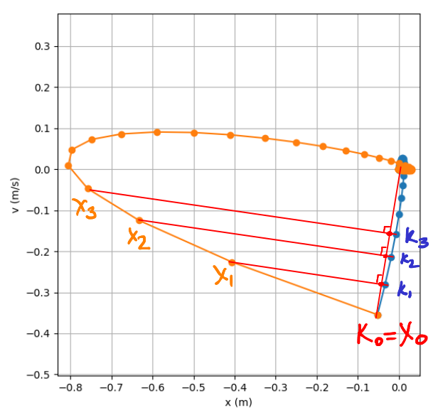
So, the theory tells us that (for a far horizon of events) the optimal control linearly depends on the remaining distance to the final goal. Last time we proved it for a one-dimensional case, in a two-dimensional case, having believed in the word. This time again I will not strictly prove, leaving it for a later conversation about Lagrange multipliers. However, it is intuitively clear that this is the case. After all, we have obtained the formula U = K * x0, where the matrix K does not depend on the state of the system, but only on the structure of the differential equation (on the matrices A and B).
That is, u_0 = k_0 * x_0. By the way, we got k_0 equal to [-0.052 -0.354]:
K = [[-0.052 -0.354]
[-0.034 -0.281]
[-0.019 -0.215]
[-0.008 -0.158]
[ 0. -0.11 ]
...
Compare this result with what I obtained with the help of the OLS and the one that was obtained by solving the Riccati equation (in the comments to the previous article). It is intuitively clear that if u0 depends linearly on x_0, then for a far horizon of events the same should be for x1.
Continuing the argument, we expect that the control u_i should be considered as u_i = k_0 * x_i. That is, the optimal control should be obtained by the scalar product of the constant vector k_0 and the residual distance to the target x_i.
But our result is exactly the opposite! We found that u_i = k_i * x_0! That is, we found the sequence k_i, which depends only on the structure of the system equation, but not on its state. And the control is obtained using the scalar product of a constant vector (the initial position of the system) and the sequence found ...
That is, if everything is good, then we should have the equality k_0 * x_i = u_i = k_i * x_0. Let's draw an illustrative graph, taking x_0 for simplicity equal to k_0. Along one axis of the graph we will postpone the coordinate of the machine, along the other the speed. Starting from one point k_0 = x_0 we get two different sequences of points k_i and x_i converging to zero coordinates.
Drawing is available here .
If roughly, then k_i * x_0 form a sequence of projections k_i onto the vector x_0. The same for k_0 * x_i, is a sequence of projections x_i on k_0. On our graph it is clearly seen that these projections coincide. Once again, this is not proof, but only an illustration.
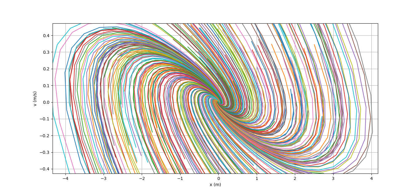
Thus, we have obtained a dynamic system of the form x_ {k + 1} = (A + BK) x_k. If the eigenvalues of the matrix A + BK are less than unity in absolute value, then this system converges to the origin for any initial x_0. In other words, the solution of this differential equation is the (matrix) exponent.
In an insane asylum, where mathematics students were brought to the session, one of them runs around with a knife and shouts: “I will differentiate everyone!”. Patients scatter, except for another math student. When the first one rushes into the chamber crying, “Differentiate!”, The second one phlegmatically remarks: “I am in the degree of X!”. The first, waving a knife: “I will differentiate by toys!”
As an illustration, I randomly selected several hundred different x_0, and drew the trajectories of our typewriter. Drawing to take here . Here is the resulting picture:
All trajectories safely converge to zero, a slight twisting of the trajectories suggests that the matrix A + BK is a rotation and contraction matrix (it has complex eigenvalues smaller than one in absolute value). If I'm not mistaken, then this picture is called a phase portrait.
Open and closed control loops
So, we cheerfully minimized our function J, and obtained the optimal control vector U0 as K * X0:
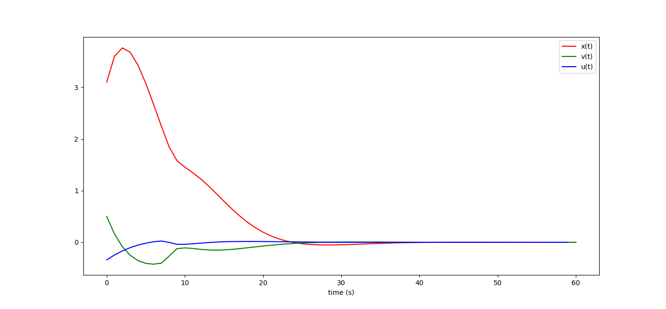
U=K*X0 X=Abar*X0 + Bbar*U Is there still a difference between considering management in the same way or as u_i = k_0 * x_i? There is a colossal, if we have unaccounted factors in the system (that is, almost always). Let's imagine that our car is not rolling on a horizontal surface, but such a slide can meet on its way:
If we calculate the optimal control without regard to this slide, then trouble can happen
(drawing here ):
The machine not only will not stop, but will go to infinity to the right altogether, I even drew a third of the x_i graphics, and then it grows linearly. If we close the control loop, then small disturbances in the dynamics of the system do not lead to catastrophic consequences:
for i in range(N): Xi = X[i*n:(i+1)*n,0] U[i*m:(i+1)*m,0] = K[0:m,:]*Xi idxslope = int((Xi[0,0]+5)/10.*1000.) if (idxslope<0 or idxslope>=1000): idxslope = 0 X[(i+1)*n:(i+2)*n,0] = A*Xi + B*U[i*m:(i+1)*m,0] + B*slope[idxslope] Building a linear observer
So, we are able to manage a dynamic system so that it strives to get to the origin. But what if we wanted the car to stop not at x = 0, but at x = 3? Obviously, it is enough to subtract the desired result from the current state x_i, and then everything is as usual. Moreover, this desired result may well not be permanent, but change over time. Can we follow another dynamic system?
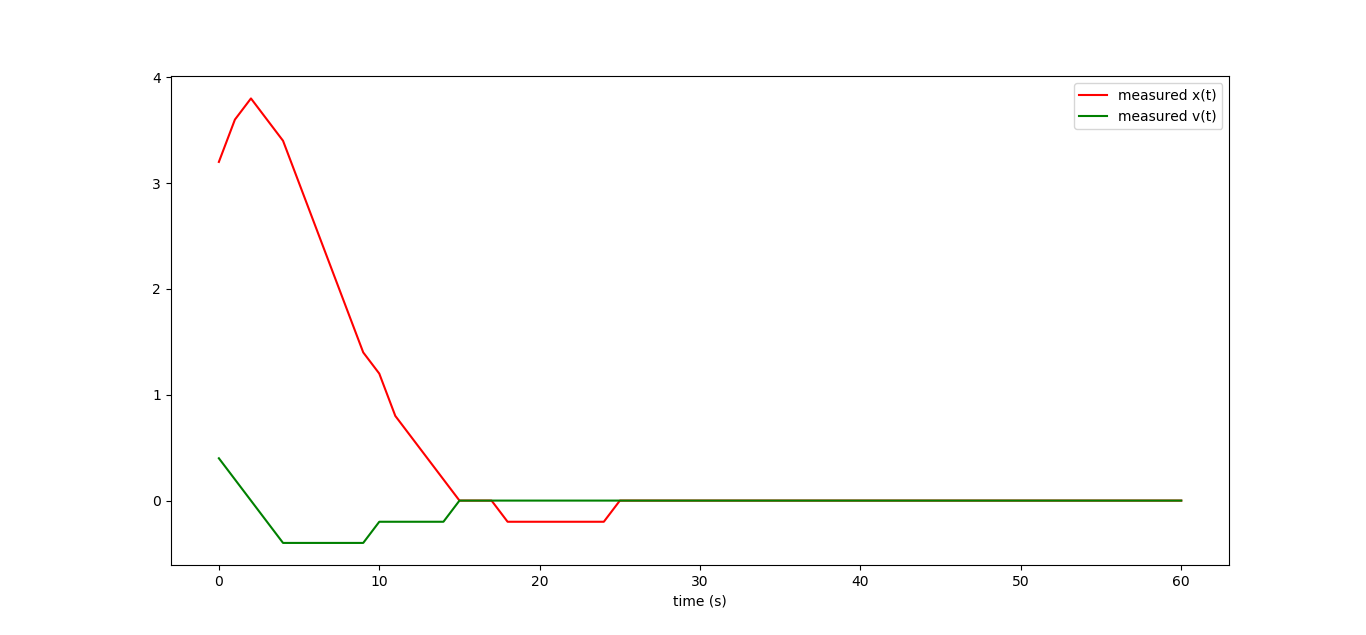
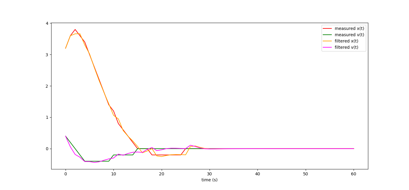
Let's assume that we do not control our typewriter directly, but at the same time we want to follow it. We measure both states of the machine with the help of some sensors that have a rather low resolution:
I just took our curves and blundered their values. Let's try to filter the noise introduced by the measurements. As usual, we arm ourselves with the smallest squares.
When you have a hammer in your hands, everything seems to be nails.
So, our machine obeys the law x_ {k + 1} = A x_k + B u_k, so let's build a diffur observer that follows the same law:
Here y_k is a corrective member, through which we will inform our observer how far we are from the real state of affairs. Like last time, we write the equation in matrix form:
Okay. Now what do we want? We want the correction terms y_k to be small, and that z_k converge to x_k:
Like last time, we express Z through Y, we equate the partial derivatives with respect to Y to zero, and we obtain the expression for the optimal corrective term:
Then vague forebodings begin to torment me ... I have already seen it somewhere! Well, let's remember how X is related to U, we get the following expression:
But this is accurate to renaming the letters for U *! And in fact, let's go back a little bit, we rushed into business too quickly. Combining the dynamics for x_k with the dynamics for z_k we get the dynamics for the error x_k-z_k.
That is, our task of tracking a typewriter is absolutely equivalent to the problem of a linear-quadratic controller. Find the optimal gain matrix, which in our case will be equal to [[-0.594, -0.673], [- 0.079, -0.774]], and we get the following observer code:
for i in range(N): Zi = Z[i*n:(i+1)*n,0] Xi = X[i*n:(i+1)*n,0] Z[(i+1)*n:(i+2)*n,0] = A*Zi + B*U[i*m:(i+1)*m,0] + np.matrix([[-0.594,-0.673],[-0.079,-0.774]])*(Zi-Xi) But the filtered curves, they are not ideal, but still closer to reality than measurements with low resolution.
The dynamics of the system is determined by the eigenvalues of the matrix [[1-0.594.1-0.673], [- 0.079.1-0.774]], which are equal (0.316 + - 0.133 i).
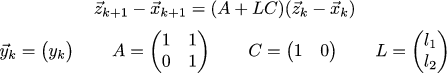
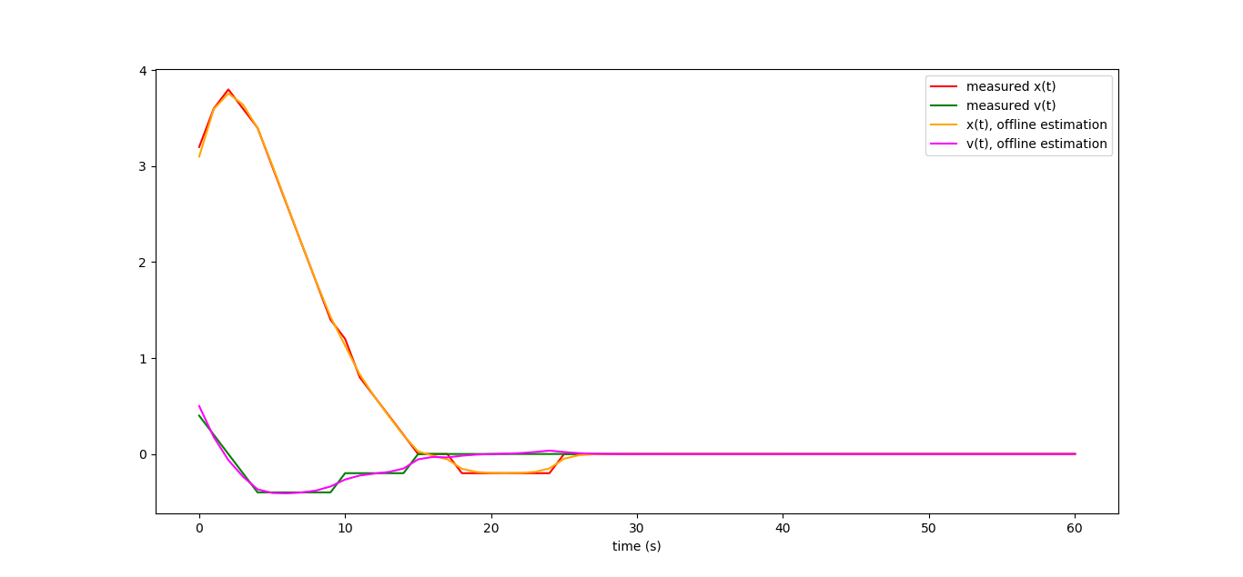
And let's go even further. Let's assume that we can measure only the position, but there is no sensor speed. Will we be able to build an observer in this case? Here we go beyond the LQR, but not too far. Let's write the following system:
Matrix C dictates to us what we can actually observe in our system. Our task is to find such a matrix L, which will allow the observer to behave well. Let's prescribe that the eigenvalues of the matrix A + LC, which describes the overall dynamics of the observer, should be about the same as the eigenvalues of the matrix from the previous example. Let's approximate the previous eigenvalues with fractions (1/3 + - 1/6 i). We write the characteristic polynomial of the matrix A + LC, and make it equal to the polynomial (x- (1/3 + 1/6 * i)) * (x- (1 / 3-1 / 6 * i). Then we solve the simplest system from linear equations, and the matrix L is found.
Calculations can be checked here , and drawing charts here .
This is how the work schedules of our observer look like, if we measure (and with a large error) only the coordinate of our machine:
From very incomplete data, we can very well restore the dynamics of the entire system! By the way, the linear observer that we built in fact is the famous Kalman filter, but we will talk about this some time next.
Question for attentive readers
If, nevertheless, to bring to the logical end the computations of Y * (code is taken here) , then the final observer curves are much much smoother (and closer to the truth!) Than those that should be equivalent to them. Why?
Source: https://habr.com/ru/post/341870/
All Articles