Create your own physical 2D engine: parts 2-4

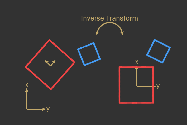
Table of contents

Part 2: engine core

• Integration
• Time stamps
• Modular architecture
  • Bodies
  • Forms
  • Forces
  • Materials
• Wide phase
  • Clipping duplicate contact pairs
  • Layer system
• Checking the intersection of half spaces

Part 3: Friction, Scene and Transition Table
')

• Friction
• Scene
• Collision transition table

Part 4: Oriented Solids

• Rotation Math
• Oriented Forms
• Collision detection
• Collision resolution

---

Part 2: engine core

In this part of the article we will add other functions to the resolution of force impulses. In particular, we consider integration, time stamps, use of modular architecture in code, and collision detection in a wide phase.

---

Introduction

In the previous post I reviewed the topic of impulse resolution . Read it first if you have not done it yet!

Let's delve into the topics covered in this article. All these topics are necessary for any more or less decent physics engine, so it is time to create new functions on top of the foundation laid in the previous post.

• Integration
• Time stamps
• Modular architecture
  • Bodies
  • Forms
  • Forces
  • Materials
• Wide phase
  • Clipping duplicate contact pairs
  • Layer system
• Checking the intersection of half spaces

---

Integration

Integration is very simple to implement, and there is a lot of information about iterative integration on the Internet. In this section, I will mainly look at the function of correct integration, and tell you the places where you can find more detailed information if you are interested.

First, you need to figure out what acceleration is. Newton's second law states:

$$

$$Equation \: 1: \\ F = ma$$

He argues that the sum of all forces acting on an object is equal to the mass of this object m multiplied by the acceleration a . m indicated in kilograms, a in meters / s, and F in newtons.

Slightly transform the equation to calculate a and get:

$$

$$Equation \: 2: \\ a = \ frac {F} {m} \\ \ therefore \\ a = F * \ frac {1} {m}$$

The next step involves accelerating to move an object from one place to another. Since the game is displayed in discrete separate frames that create the illusion of animation, it is necessary to calculate the places of each of the positions of these discrete steps. For a more detailed analysis of these equations, see the Erin Kutto integration demo with GDC 2009 and the Hannu supplement to the Euler symplectic method to improve stability in low FPS environments .

The integration with the explicit Euler method is shown in the following code snippet, where x is the position and v is the speed. It is worth noting that, as explained above, 1/m * F is the acceleration:

 //    x += v * dt v += (1/m * F) * dt 

dt here denotes the delta (increment) of time. Δ is a delta symbol, and can literally be read as a “change in magnitude,” or written as Δ t . So when you see dt , it can be read as a “time change”. dv is “speed change”.

This system will work and is usually used as a starting point. However, it has numerical inaccuracies that can be eliminated without unnecessary trouble. Here is an algorithm called Euler's symplectic method:

 //    v += (1/m * F) * dt x += v * dt 

Notice that I just converted the order of two lines of code — see Hannu, the above article .

This post explains the numerical inaccuracies of Euler’s explicit method, but keep in mind that Hannu is starting to consider RK4, which I personally do not recommend: gafferongames.com: inaccuracy of Euler’s method .

These simple equations are enough to move all objects with linear velocity and acceleration.

---

Time stamps

Since games are displayed at discrete time intervals, we need a method of controlled time manipulation between these steps. Have you ever seen a game that runs on different computers at different speeds? This is an example of a game that runs at a speed that depends on the power of the computer.

We need a way to ensure that the physics engine is executed only after a certain amount of time has passed. Thus, the dt used in the calculations will always remain the same number. If everywhere in the code we use the exact constant value dt , then our physics engine will turn into deterministic , and this property of it will be known as a constant time stamp . This is a very handy thing.

A deterministic physics engine is one that, with the same input, will always do the same thing. This is necessary in many types of games in which the gameplay must be clearly tied to the behavior of the physics engine. In addition, it is necessary to debug our engine, because to detect errors in the behavior of the engine, it must be constant.

First, let's look at a simple version of the permanent time stamp. Here is an example:

 const float fps = 100 const float dt = 1 / fps float accumulator = 0 //   -  float frameStart = GetCurrentTime( ) //   while(true) const float currentTime = GetCurrentTime( ) //  ,      accumulator += currentTime - frameStart( ) //     frameStart = currentTime while(accumulator > dt) UpdatePhysics( dt ) accumulator -= dt RenderGame( ) 

This code waits and renders the game until enough time has passed to update the physics. Elapsed time is recorded, and discrete blocks of time the size of dt are taken from the accumulator and processed by physics. This ensures that under any conditions the same value is transmitted to physics, and that the value transferred to physics is an exact representation of the actual time passed in real life. The dt blocks are removed from the accumulator until the accumulator becomes smaller than the dt block.

Here we can fix a couple of problems. The first is related to how long it takes to update the physics: what happens if the physics update takes too much time and with each game cycle accumulator will be more and more? This is called the "death spiral." If this problem is not solved, the engine will quickly come to a complete stop if the calculation of physics is not fast enough.

To solve the problem, the engine needs fewer physics updates if the accumulator becomes too large. One of the easiest ways to do this is to limit the accumulator so that it cannot be greater than any arbitrary value.

 const float fps = 100 const float dt = 1 / fps float accumulator = 0 //   -  float frameStart = GetCurrentTime( ) //   while(true) const float currentTime = GetCurrentTime( ) //  ,      accumulator += currentTime - frameStart( ) //     frameStart = currentTime //       dt,   //    UpdatePhysics  //   . if(accumulator > 0.2f) accumulator = 0.2f while(accumulator > dt) UpdatePhysics( dt ) accumulator -= dt RenderGame( ) 

Now, if the game performing this cycle finds it simple for some reason, then physics will not drag itself into the death spiral. The game will simply run a little slower, as it should.

The next problem is much smaller than the death spiral. This cycle receives dt blocks from accumulator , until accumulator becomes less than dt . This is great, but in accumulator is still some time left. That is the problem.

Assume that in the accumulator each frame remains 1/5 of the dt block. On the sixth frame in accumulator will be enough time remaining to perform one more physics update for all other frames. This will result in a slightly larger discrete jump in time, approximately at one frame per second, or so, and this can be very noticeable in the game.

To solve this problem, you must use linear interpolation . It sounds scary, but do not be afraid - I will show the implementation. If you want to understand how to implement it, then there are many resources on the Internet devoted to linear interpolation.

 //    a  0  1 //  t1  t2 t1 * a + t2(1.0f - a) 

With this code we can interpolate (approximate) the place in which we can be between two different time intervals. This position can be used to render the game state between two physics updates.

Using linear interpolation, you can render the engine at a speed different from the execution of the physical engine. This allows you to elegantly handle the remainder of the accumulator of physics updates.

Here is a complete example:

 const float fps = 100 const float dt = 1 / fps float accumulator = 0 //   -  float frameStart = GetCurrentTime( ) //   while(true) const float currentTime = GetCurrentTime( ) //  ,      accumulator += currentTime - frameStart( ) //     frameStart = currentTime //       dt,   //    UpdatePhysics  //   . if(accumulator > 0.2f) accumulator = 0.2f while(accumulator > dt) UpdatePhysics( dt ) accumulator -= dt const float alpha = accumulator / dt; RenderGame( alpha ) void RenderGame( float alpha ) for shape in game do //      Transform i = shape.previous * alpha + shape.current * (1.0f - alpha) shape.previous = shape.current shape.Render( i ) 

Thus, all objects in the game can be drawn at variable moments between the discrete time stamps of physics. This allows you to elegantly handle all errors and the accumulation of time. In fact, the rendering will be performed a little later than the computed physics, but when you watch the game, the whole movement is remarkably smoothed by interpolation.

The player will never guess that rendering is constantly lagging behind physics, because he will know only what he sees, and he will see perfectly smooth transitions from one frame to another.

You may ask yourself: why do we not interpolate from the current position to the next? I tried to do so and it turned out that this requires that the rendering "guessed" where the objects will be in the future. Objects in a physics engine can often suddenly change their motion, for example, during collisions, and when such drastic changes occur, objects are teleported to another place due to inaccurate interpolations for the future.

---

Modular architecture

Each physical object requires several properties. However, the parameters for each specific object may differ slightly. We need a smart way to organize all of this data, and we will assume that for such ordering it is desirable to write as little code as possible. In this case, we have a modular architecture.

The phrase "modular architecture" may sound pathetic and pereuslozhenno, but in fact it is quite logical and quite simple. In this context, “modular architecture” simply means that we can break up physical objects into separate parts so that they can be connected and separated in a convenient way.

Bodies

A physical body is an object containing all the information about a particular physical object. It will store the form (or forms) that make up the object, data on mass, transformation (position, turn), speed, torque, etc. Here is what the body will look like:

 struct body { Shape *shape; Transform tx; Material material; MassData mass_data; Vec2 velocity; Vec2 force; real gravityScale; }; 

This is a great starting point for creating the structure of the physical body. Here logical decisions are made to create a good code structure.

First, it is worth noting that the form is placed in the body with a pointer. This creates a weak connection between the body and its form. The body can contain any shape, and the shape of the body can be arbitrarily changed. In fact, a body can be represented by several forms, and such a body will be called “composite”, because it consists of several forms. (In this tutorial, I will not consider composite bodies.)


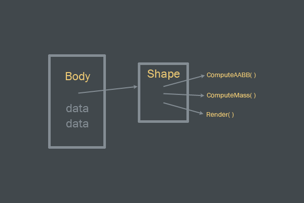
Interface body and shape.

The shape itself is responsible for calculating the boundary shapes, calculating the mass based on density, and rendering.

mass_data is a small data structure for storing mass-related information:

 struct MassData { float mass; float inv_mass; //   (  ) float inertia; float inverse_inertia; }; 

It is very convenient to store in a single structure all values ​​related to mass and inertia. Mass should never be set manually - the mass must always be calculated from the form itself. Mass is a rather unintuitive type of value, and manually setting it will take a long time to fine-tune. It is defined as follows:

$$

$$Equation 3: \\ mass = density * volume$$

When a designer needs a form to be more “massive” or “heavy”, then he should change the density of the form. This density can be used to calculate the mass of a form using its volume. This is the right way to act in such a situation, because the density is not affected by the volume and it never changes during the execution of the game (unless provided with a special code).

Some of the examples of shapes, such as AABB and circles, can be found in the previous part of the tutorial .

Materials

All this talk about mass and density leads us to the question: where is the density value stored? It is in the Material structure:

 struct Material { float density; float restitution; }; 

After setting the material values, this material can be transferred to the shape of the body so that the body can calculate the mass.

The last thing worth mentioning is gravity_scale . Scaling gravity for different objects is very often useful when fine-tuning the gameplay, so each body should add this value specifically for this task.

Useful settings for the most common materials can be used to create the enumeration value of the Material object:

 Rock Density : 0.6 Restitution : 0.1 Wood Density : 0.3 Restitution : 0.2 Metal Density : 1.2 Restitution : 0.05 BouncyBall Density : 0.3 Restitution : 0.8 SuperBall Density : 0.3 Restitution : 0.95 Pillow Density : 0.1 Restitution : 0.2 Static Density : 0.0 Restitution : 0.4 

Forces

We need to discuss another aspect in the body structure. This is a data item called force . At the beginning of each physics update, this value is zero. Other effects of the physics engine (for example, gravity) add to this data element force Vec2 vectors. Immediately before integration, all these forces are used to calculate the acceleration of the body and are applied at the integration stage. After integration, this force data item is set to zero.

This allows an object to act on any number of forces, and to apply new types of forces to objects, no new code should be written.

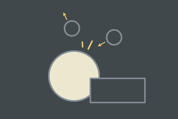
Let's take an example. Suppose we have a small circle, which is a very heavy object. This small circle flies around the game world, and it is so heavy that it constantly slightly attracts other objects. Here is a rough pseudocode to demonstrate this:

 HeavyObject object for body in game do if(object.CloseEnoughTo( body ) object.ApplyForcePullOn( body ) 

The ApplyForcePullOn() function can refer to a small force that attracts a body to a HeavyObject only if the body is close enough.


Two objects drawn to a larger object moving past them. The forces of attraction depend on the distance to a large rectangle.

It does not matter how much force is applied to the force body, because they are summed up into a single common vector of this body. This means that two forces acting on one body can potentially balance each other.

---

Wide phase

In the previous article in the series, we introduced collision recognition procedures. These procedures are in fact independent of what is called the “narrow phase”. The differences between the wide and narrow phases can be quite easily found on Google.

(In short: we use the wide collision recognition phase to determine which pairs of objects can collide, and then the narrow collision recognition phase to check if they really collide.)

I want to give an example of code with an explanation of how to implement a wide phase of computing pairs of the algorithm with time complexity $$$O (n ^ 2)$ .

$$$O (n ^ 2)$ means that the time spent checking each pair of potential collisions depends on the square of the number of objects. Here, the “O” notation is large .

Since we work with pairs of objects, it will be useful to create a similar structure:

 struct Pair { body *A; body *B; }; 

The wide phase should collect a group of possible collisions and save them all in the structures of the Pair . These pairs can then be transferred to another part of the engine (narrow phase) for later resolution.

Example of a wide phase:

 //   . //        . void BroadPhase::GeneratePairs( void ) { pairs.clear( ) //    AABB,    //       AABB A_aabb AABB B_aabb for(i = bodies.begin( ); i != bodies.end( ); i = i->next) { for(j = bodies.begin( ); j != bodies.end( ); j = j->next) { Body *A = &i->GetData( ) Body *B = &j->GetData( ) //      if(A == B) continue A->ComputeAABB( &A_aabb ) B->ComputeAABB( &B_aabb ) if(AABBtoAABB( A_aabb, B_aabb )) pairs.push_back( A, B ) } } } 

The code above is quite simple: we check every body with every other body, and skip checking for collisions with ourselves.

Duplicate clipping

In the last section there is one problem: many duplicate pairs will be returned! These duplicates must be removed from the results. If you do not have a sorting library at hand, this will require familiarity with sorting algorithms. If you are writing in C ++, then you are lucky:

 //      sort( pairs, pairs.end( ), SortPairs ); //       { int i = 0; while(i < pairs.size( )) { Pair *pair = pairs.begin( ) + i; uniquePairs.push_front( pair ); ++i; //  ,  ,      while(i < pairs.size( )) { Pair *potential_dup = pairs + i; if(pair->A != potential_dup->B || pair->B != potential_dup->A) break; ++i; } } } 

After sorting all pairs in a certain order, we can assume that all pairs in the container have a duplicate in the neighborhood. Place all unique pairs in the new uniquePairs container, and the work on duplicating duplicates is completed.

The last thing worth mentioning is the predicate SortPairs() . This SortPairs() function is used for sorting. It might look like this:

 bool SortPairs( Pair lhs, Pair rhs ) { if(lhs.A < rhs.A) return true; if(lhs.A == rhs.A) return lhs.B < rhs.B; return false; } 

The lhs and rhs members can be decoded as the “left hand side” (left side) and the “right hand side” (right side). These terms are usually used to work with parameters of functions, in which elements can be logically considered as the left and right sides of an equation or algorithm.

Layer system

The layer system is needed so that different objects never collide with each other. It is necessary that bullets flying from certain objects do not affect other specific objects. For example, players of one team with missiles must deal damage to enemies, but not to each other.


Explanation of the system of layers: some objects collide with each other, others do not.

The layer system is best implemented using bitmasks . To learn how bitmasks are used in engines, see for a brief introduction to bitmasks for programmers , the Wikipedia page and the Filtering section in the Box2D tutorial .

The layer system is implemented in a wide phase. Here I will simply insert a ready-made example of a wide phase:

 //   . //        . void BroadPhase::GeneratePairs( void ) { pairs.clear( ) //    AABB,    //       AABB A_aabb AABB B_aabb for(i = bodies.begin( ); i != bodies.end( ); i = i->next) { for(j = bodies.begin( ); j != bodies.end( ); j = j->next) { Body *A = &i->GetData( ) Body *B = &j->GetData( ) //      if(A == B) continue //     if(!(A->layers & B->layers)) continue; A->ComputeAABB( &A_aabb ) B->ComputeAABB( &B_aabb ) if(AABBtoAABB( A_aabb, B_aabb )) pairs.push_back( A, B ) } } } 

The layer system is highly efficient and very simple.

---

Intersection of half spaces

A half-space can be viewed in 2D as one side of a straight line. Determining whether a point is on one or the other side of the line is a fairly common task, and when implementing your own physics engine you need to understand it well. It is very bad that this topic, as it seems to me, is not disclosed anywhere on the Internet in detail, and we will fix it!

The general equation of a straight line in 2D has the following form:

$$

$$\: 4:\\ \: : ax + by + c = 0\\ \: \: : \begin{bmatrix} a \\ b \\ \end{bmatrix}$$

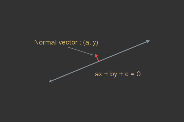
Note that despite its name, the normal vector is not always necessarily normalized (that is, it does not necessarily have a length of 1).

To determine whether a point is on a certain side of a line, all we need to do is substitute a point into variables xand yequations and check the sign of the result. A result of 0 will mean that the point is on a straight line, and a positive / negative value means different sides of a straight line.

And that is all! Knowing this, from point to line is the result of a previous check. If the normal vector is not normalized, then the result is scaled by the magnitude of the normal vector.

---

Conclusion

To this stage you can create a complete, albeit very simple physics engine from scratch. In the following sections, we will look at more complex topics: friction: orientation, and the dynamic tree AABB.

Part 3: Friction, Scene and Transition Table

In this part of the article we will cover the following topics:

• Friction
• Scene
• Collision transition table

---

Video demo

Here is a brief demo of what we will work on in this part:

---

Friction

— . , , , .

— . : « », , , .

:


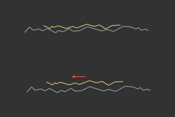
The interactions between the bodies are quite interesting, and the repulsion in case of collisions looks realistic. However, when objects land on a fixed platform, they all seem to repel and slide off the edges of the screen. So it turns out because of the lack of friction simulation.

Impulses of power, again?

, j , . jnormal jN , .

, jtangent jT . . , , , . , 3D .

Friction is quite simple, and we can again use our previous equation for j, just replace all the normals nwith a tangent vector t.

$$

$$\: 1:\\ j = \frac{-(1 + e)(V^{B}-V^{A})\cdot n)} {\frac{1}{mass^A} + \frac{1}{mass^B}}$$

Replace nwith t:

$$

$$\:2:\\ j = \frac{-(1 + e)((V^{B}-V^{A})\cdot t)} {\frac{1}{mass^A} + \frac{1}{mass^B}}$$

t n , , 2.

, t . — , , . — , !

, . . , «» . , «» .


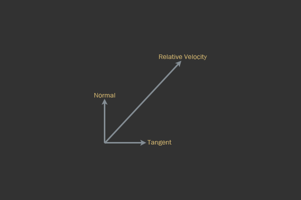
Different types of vectors in the time frame of a collision of solids.

As was briefly described above, friction will be a vector directed in the opposite direction from the tangent vector. This means that the direction in which we apply friction can be calculated directly, because the normal vector is in the recognition of collisions.

If we know this, then the tangent vector is (where nis the normal to the collision):

$$

$$V^R = V^{B}-V^{A} \\ t = V^R - (V^R \cdot n) * n$$

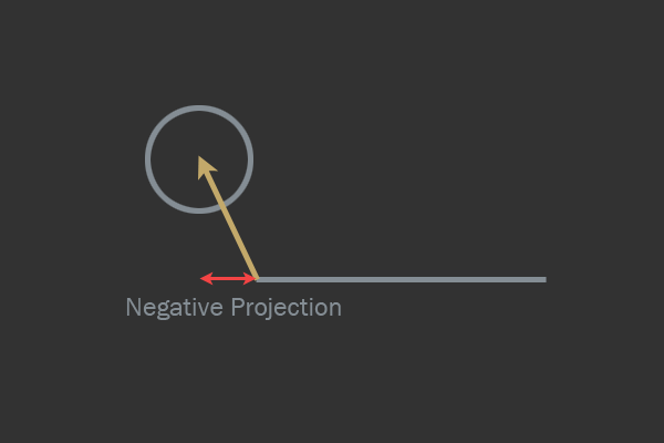
To determine the amount of friction jt, we need only directly calculate the value of the above equations. Soon we will look at other tricks after calculating this value, so this is not the only thing needed for our resolution of collisions:

 //      //   (    ,     //      ) Vec2 rv = VB - VA //    Vec2 tangent = rv - Dot( rv, normal ) * normal tangent.Normalize( ) //  ,     float jt = -Dot( rv, t ) jt = jt / (1 / MassA + 1 / MassB) 

The above code directly corresponds to Equation 2. Again, it is important to understand that the friction vector points in the direction opposite to the tangent vector. Therefore, we must add a minus sign when the scalar product of relative velocity is tangential to calculate the relative velocity along the tangent vector. The minus sign reverses the tangential velocity and suddenly points in the direction in which the friction should be approximated.

Amonton-Coulomb Law

The Amonton-Coulomb Law is that part of the friction simulation in which most programmers have difficulty. I myself had to study it long enough to find the right way to model it. The trick is that the Amonton-Coulomb law is an inequality.

It reads:

$$

$$\:3: \\ F_f <= \mu F_n$$

, , μ ( ).

— j , . jt ( ) μ , jt . , , μ . «» - , , μ .

The whole point of Amonton-Coulomb's law is to follow this restriction procedure. Such a restriction turns out to be the most difficult part of the friction simulation for resolution on the basis of impulses of force — there is nowhere to find documentation on it, but now we will fix it! In most of the articles I have found on this topic, friction is either completely discarded, or is mentioned briefly, and the restriction procedures are implemented incorrectly (or do not exist at all). I hope you now realize that a correct understanding of this part is very important.

Before explaining something, let's fully implement the constraint. The code block below is the previous example with the finished limiting procedure and the application of a friction force pulse:

 //      //   (    ,     //      ) Vec2 rv = VB - VA //    Vec2 tangent = rv - Dot( rv, normal ) * normal tangent.Normalize( ) //  ,     float jt = -Dot( rv, t ) jt = jt / (1 / MassA + 1 / MassB) // PythagoreanSolve = A^2 + B^2 = C^2,  C   A  B //           float mu = PythagoreanSolve( A->staticFriction, B->staticFriction ) //         Vec2 frictionImpulse if(abs( jt ) < j * mu) frictionImpulse = jt * t else { dynamicFriction = PythagoreanSolve( A->dynamicFriction, B->dynamicFriction ) frictionImpulse = -j * t * dynamicFriction } //  A->velocity -= (1 / A->mass) * frictionImpulse B->velocity += (1 / B->mass) * frictionImpulse 

:

$$

$$\:4: \\ Friction = \sqrt[]{Friction^2_A + Friction^2_B}$$

, - , . , . , . : , .

, jt , «» - . j , , .

- . .

- : , « ». , , . , .

- . :


.

, , , . , , . , .

. : — , .

jt . jt ( ), , , , jt .

, jt , , « », , .

---

If you carefully read the section "Friction", then congratulations! You have completed the most difficult (in my opinion) part of the whole tutorial.

The class is Sceneused as a container for everything related to the physical simulation scenario. It causes and uses the results of all broad phases, contains all solids, performs collision checks and causes their resolution. It also combines all active objects. The scene also interacts with the user (for example, a programmer using a physics engine).

Here is an example of how the scene structure might look like:

 class Scene { public: Scene( Vec2 gravity, real dt ); ~Scene( ); void SetGravity( Vec2 gravity ) void SetDT( real dt ) Body *CreateBody( ShapeInterface *shape, BodyDef def ) //        ( ). void InsertBody( Body *body ) //     void RemoveBody( Body *body ) //      void Step( void ) float GetDT( void ) LinkedList *GetBodyList( void ) Vec2 GetGravity( void ) void QueryAABB( CallBackQuery cb, const AABB& aabb ) void QueryPoint( CallBackQuery cb, const Point2& point ) private: float dt //     float inv_dt // ,      LinkedList body_list uint32 body_count Vec2 gravity bool debug_draw BroadPhase broadphase }; 

Scene . , . BodyDef — , , - .

Step() . , . , .

AABB , AABB. , .

---

We need a simple way to select the called collision function depending on the type of two different objects.

In C ++, I know two main ways: double dispatch and a two-dimensional transition table. In my tests, I found out that the two-dimensional table is more optimal, so I will consider its implementation in detail. If you plan on using non-C and non-C ++, then I’m sure that, like a function pointer table, you can create an array of functions or functional objects (and this is another reason for choosing transition tables, and not other options that are specific to C ++).

The transition table in C or C ++ is a table of function pointers. Indices, which are arbitrary names or constants, are used as a table index and to call a specific function. Using a one-dimensional conversion table might look like this:

 enum Animal { Rabbit Duck Lion }; const void (*talk)( void )[] = { RabbitTalk, DuckTalk, LionTalk, }; //         talk[Rabbit]( ) //   RabbitTalk 

The above code actually simulates what the C ++ language itself implements through . However, in C ++ only one-dimensional calls to virtual functions are implemented. A two-dimensional table can be built manually.

Here is the pseudocode for a two-dimensional transition table for calling collision procedures:

 collisionCallbackArray = { AABBvsAABB AABBvsCircle CirclevsAABB CirclevsCircle } //        //   A and B,       //    AABB   collisionCallbackArray[A->type][B->type]( A, B ) 

! .

, AABBvsCircle CirclevsAABB . ! , . .

---

Conclusion

, ! , . , .

: . , , .

, .

4:

So, we have considered the resolution of impulses of force , the architecture of the core and friction. In this last part of the tutorial, I will cover a very interesting topic: orientation.

In this part we will talk about the following topics:

• Rotation Math
• Oriented Forms
• Collision detection
• Collision resolution

---

Code example

I created a small example of the C ++ engine, and I recommend that you study the source code while reading the article, because many implementation details did not fit into the article itself.


This GitHub repository contains an example engine itself along with a Visual Studio 2010 project. For convenience, GitHub allows you to view the code without having to download it.

Other related articles

• Philip Difenderfer forks the repository to create a Java version of the engine!

---

Orientation Math

Mathematics related to rotations in 2D is quite simple, however, to create everything valuable in a physics engine, knowledge of the subject is required. Newton's second law states:

$$

$$\: 1:\\ F = ma$$

There is a similar equation relating specifically to rotational force and angular acceleration. However, before getting acquainted with these equations, it is worthwhile to briefly describe the vector product in two-dimensional space.

Vector product

Vector artwork in 3D is a well-known operation . However, a vector product in 2D can be quite confusing, because it actually does not have a convenient geometric interpretation.

A vector product in 2D, as opposed to a version in 3D, does not return a vector, but a scalar. This scalar product actually determines the magnitude of the orthogonal vector along the Z axis, as if the vector product is performed in 3D. In a sense, a vector product in 2D is a simplified version of a vector product in 3D, because it is an extension of three-dimensional vector mathematics.

, : . , , , : $$$a \ times b$ — , $$$b \times a$ . .

, 2D . , , . :

 //       float CrossProduct( const Vec2& a, const Vec2& b ) { return ax * by - ay * bx; } //   ( )    //   a   s,    Vec2 CrossProduct( const Vec2& a, float s ) { return Vec2( s * ay, -s * ax ); } Vec2 CrossProduct( float s, const Vec2& a ) { return Vec2( -s * ay, s * ax ); } 

As we know from the previous parts, this equation denotes the relationship between the force acting on the body, with the mass and the acceleration of this body. He has an analogue for rotation:

$$

$$\: 2:\\ T = r \: \times \: \omega$$

$$T stands fortorque. Torque is the force of rotation.$T$

$$r is a vector from the center of mass (CM) to a specific point of the object.$r$$$r can be considered the "radius" from the CM to the point. Each unique point of the object needs its own value.$r$$$r for substitution in Equation 2.$r$

$$ o m e g a is called “omega” and means rotation speed. This ratio will be used to integrate the angular velocity of the solid body.It is important to understand that linear velocity is the speed of the CM of a solid body. In the previous part, all objects did not have rotation components, therefore the linear velocity of the CM was the same as the speed of all points of the body. When an orientation is added, points remote from the CM rotate faster than those closest to the CM. This means that we need a new equation to find the velocity of the point of the body, because the bodies can now rotate and move simultaneously.Use the following equation to understand the relationship between the point of the body and the speed of this point:$\ omega$

$$

$$\: 3:\\ \omega = r \: \times v$$

$$$v$ . , $$$r$ and $$$v$ .

3 :

$$

$$\: 4:\\ v = \omega \: \times r$$

, . , , . , , , , $$$r$ .

Z. , . , , , . « » .

- , — . , .

, , . , , . . .

. , :

 struct RigidBody { Shape *shape //   Vec2 position Vec2 velocity float acceleration //   float orientation //  float angularVelocity float torque }; 

. ( ):

 const Vec2 gravity( 0, -10.0f ) velocity += force * (1.0f / mass + gravity) * dt angularVelocity += torque * (1.0f / momentOfInertia) * dt position += velocity * dt orient += angularVelocity * dt 

, , . , , , , , .

Mat22

As shown above, the orientation should be stored as one value in radians, however, it is often more convenient for some figures to store a small rotation matrix.

A good example of this is the oriented boundary rectangle (Oriented Bounding Box, OBB). OBB consists of width and height, which can be represented as vectors. These two dimension vectors can be rotated using a two-by-two rotation matrix representing the OBB axes.

I recommend adding a matrix class to your math library Mat22. I myself use my own small math library, which is in the open source demo. Here is an example of what an object might look like:

 struct Mat22 { union { struct { float m00, m01 float m10, m11; }; struct { Vec2 xCol; Vec2 yCol; }; }; }; 

: , , , Vec2 , Mat22 , .

x y . :

 Mat22 m( PI / 2.0f ); Vec2 r = m.ColX( ); //    x 

: x y . , , . , .

:

 Mat22::Mat22( const Vec2& x, const Vec2& y ) { m00 = xx; m01 = xy; m01 = yx; m11 = yy; } //  Mat22::Mat22( const Vec2& x, const Vec2& y ) { xCol = x; yCol = y; } 

Since the most important operation of the rotation matrix is ​​to perform turns based on the angle, it is important to have possible to create a matrix from the angle and multiply the vector by this matrix (to rotate the vector counterclockwise by the angle the matrix was created with):

 Mat2( real radians ) { real c = std::cos( radians ); real s = std::sin( radians ); m00 = c; m01 = -s; m10 = s; m11 = c; } //   const Vec2 operator*( const Vec2& rhs ) const { return Vec2( m00 * rhs.x + m01 * rhs.y, m10 * rhs.x + m11 * rhs.y ); } 

For the sake of brevity, I will not deduce why the anti-clockwise rotation matrix has the following form:

 a = angle cos( a ), -sin( a ) sin( a ), cos( a ) 

However, it is important to at least know that this is the kind of rotation matrix. More information about the rotation matrix can be found on the page in Wikipedia .

Other related articles

• Create your own software 3D engine , part 2: linear transformations

---

Transformation to base

. — , . , .

, . , . ( ), . Mat22 . u .

.

, . . !


( ) .

, , , AABB OBB, .

, . , , .

---

. . .

. ( ) (Separating Axis Theorem, SAT).

, GDC 2013 ( ).

, — .

— , . , .

. , :

 //       Vec2 GetSupport( const Vec2& dir ) { real bestProjection = -FLT_MAX; Vec2 bestVertex; for(uint32 i = 0; i < m_vertexCount; ++i) { Vec2 v = m_vertices[i]; real projection = Dot( v, dir ); if(projection > bestProjection) { bestVertex = v; bestProjection = projection; } } return bestVertex; } 

. , . .

( A B). , A .



, . . , , .

. , .

, GetSupport :

 real FindAxisLeastPenetration( uint32 *faceIndex, PolygonShape *A, PolygonShape *B ) { real bestDistance = -FLT_MAX; uint32 bestIndex; for(uint32 i = 0; i < A->m_vertexCount; ++i) { //      A Vec2 n = A->m_normals[i]; //     B  -n Vec2 s = B->GetSupport( -n ); //      A,   //   B Vec2 v = A->m_vertices[i]; //     (   B) real d = Dot( n, s - v ); //    if(d > bestDistance) { bestDistance = d; bestIndex = i; } } *faceIndex = bestIndex; return bestDistance; } 

, , , ( , ).

, A B.

, . , ( Box2D , Blizzard) , .

. .

, , .

, . , , : .

, , .

. , . :


.

, , , . , . , , .

, . .

, , . , , 90 , . .


.

90 , . 90 , . , , , , .

, . , 90 , , .

---

: . , , .

. .

, :

$$

$$\: 5: \\ j = \frac{-(1 + e)((V^{A} - V^{B}) * t)}{\frac{1}{mass^{A}} + \frac{1}{mass^{B}}}$$

, :

$$

$$\: 6: \\ j = \frac{-(1 + e)((V^{A} - V^{B}) * t)}{\frac{1}{mass^{A}} + \frac{1}{mass^{B}} + \frac{(r^{A} \times t)^{2}}{I^{A}} + \frac{(r^{B} \times t)^{2}}{I^{B}}}$$

$$$r$ — «», . .

, :

$$

$$\: 7: \\ V' = V + \omega \times r$$

:

 void Body::ApplyImpulse( const Vec2& impulse, const Vec2& contactVector ) { velocity += 1.0f / mass * impulse; angularVelocity += 1.0f / inertia * Cross( contactVector, impulse ); } 

---

Conclusion

. , , , .

, ! — , .