Barnes-Hut t-SNE and LargeVis: visualization of large amounts of data

With data sets of millions of instances in machine learning problems, you’ll not surprise anyone for a long time. However, few people wonder how to visualize these titanic layers of information. When the dataset size exceeds one million, it becomes rather sad to use the standard t-SNE; It remains to be played with downsampling or even limited to coarse statistical tools. But for each task there is a tool. In my article, I would like to consider two algorithms that overcome the barrier of quadratic complexity: the already well-known Barnes-Hut t-SNE and the new contender for the “golden hammer infovis'a” LargeVis.


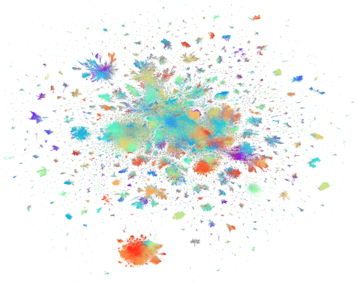
(This is not a picture of an abstract artist, but a visualization of LiveJournal dataset from a bird's-eye view)

t-SNE with modifications

Although t-SNE is about ten years old, you can safely say that it has already been tested by time. He is popular not only among experienced adepts of data science, but also among authors of popular science articles . About him already wrote on Habré; also about this visualization algorithm there are many good articles on the Internet.

However, almost all of these articles talk about standard t-SNE. I will remind him in brief:
')

1. Calculate a pair of data points for each pair. $$$x_i, x_j \ in X$ Their similarity to each other in the original space using the Gaussian kernel:
   
   

   $$

   $$p_ {j | i} = \ frac {\ exp {(- \ left \ | x_i - x_j \ right \ | ^ 2 / (2 \ sigma ^ 2_i)}} {\ sum_ {k \ neq i} (\ exp {(- \ left \ | x_i - x_k \ right \ | / (2 \ sigma ^ 2_i)})}$$

   $$

   $$p_ {ij} = \ frac {p_ {j | i} + p_ {i | j}} {2}$$
2. For each pair of display points, express their similarity in the visualization space using the t-distribution core
   
   

   $$

   $$q_ {ij} = \ frac {(1 + \ left \ | y_i - y_j \ right \ | ^ 2) ^ {- 1}} {\ sum_ {k \ neq m} (1 + \ left \ | y_k - y_m \ right \ | ^ 2) ^ {- 1}}$$
3. Build the objective function and minimize it relative to $$$y$ using gradient descent
   
   

   $$

   $$C (y) = KL (P || Q) = \ sum_ {i \ neq j} {p_ {ij} \ log {\ frac {p_ {ij}} {q_ {ij}}}}$$

Where $$$KL (P || Q)$ - Kullback-Leibler divergence.

Intuitively for a three-dimensional case, this can be represented as follows. You have $$$N$ billiard balls. You label them and hang them by the threads to the ceiling. Threads of different sizes, so now in the three-dimensional space of your room dataset hanging from $$$N$ elements with $$$d = 3$ . You connect each pair of balls with an ideal spring so that the springs are exactly the same length that you need (they do not sag, but they are not too tight). The stiffness of the springs is chosen as follows: if there are no other balls next to a ball, all the springs are more or less weak. If exactly one ball is a neighbor, and all the others are far away, then this neighbor will have a very rigid spring, and all the others will be weak. If there are two neighbors, before the neighbors there will be hard springs (but weaker than in the previous case), and to all the others - even weaker. And so on.

Now you take the resulting structure and try to place it on the table. Even if a three-dimensional object consists of freely moving nodes, in general it cannot be placed on a plane (imagine how you are pressing a tetrahedron to the table), so you simply position it so that the tension or tension of the springs is as low as possible. We do not forget to make a correction for the fact that in a two-dimensional space each ball will have fewer neighbors, but more neighbors at an average distance (remember the cube-square law). Most of the springs are so weak that they can not be taken into account at all, but the elements connected by strong springs are better placed side by side. You move in small steps, moving from an arbitrary initial configuration, slowly reducing the tension of the springs. The better you can restore the original tension of the springs at their current tension, the better.

(forgot for a second that we know that the initial tension of the springs is zero)
(Did I mention that these are magic balls and springs that pass through each other?)
(why bother with such nonsense at all? - left as an exercise for the reader)

So, modern data science packages do not quite realize this. Standard t-SNE is complex $$$O (N ^ 2)$ . As a result of recent studies , it turned out that this is redundant, and almost the same result can be achieved in $$$O (N \ log {N})$ operations.

First, count everything in the first step. $$$p_ {ij}$ it seems obviously redundant. Most of them will still be zero. Limit this number: find the k nearest neighbors of each data instance, and calculate $$$p_ {ij}$ honestly only for them; for the rest we set zero. Accordingly, the sum in the denominator of the corresponding formula will be calculated only by these elements. The question is: how to choose this number of neighbors? The answer is surprisingly simple: we already have a parameter responsible for the relationship between the global and the local structure of the algorithm - $$$u$ perplexity! Its characteristic values ​​lie in the range from 5 to 50, and, the more dataset, the more perplexity. Just what you need. With the help of the VP-tree, you can find a sufficient number of neighbors for $$$O (unN \ log {N})$ of time. If we continue the analogy with springs, it’s not like connecting all the balls in pairs, but for each ball to hang the springs up to, say, its five nearest neighbors.

Secondly…

Barnes-Hut algorithm

Let's digress a bit to discuss Barnes-Hut. About this algorithm there was no separate article on Habré, and here is just an excellent reason to tell about it.

Probably everyone is familiar with the classical gravitational problem of N bodies: based on given masses and initial coordinates of N cosmic bodies and the well-known law of their interaction, construct functions that show the coordinates of objects at all subsequent points in time. Its solution is not expressed in terms of algebraic functions that are familiar to us, but can only be found numerically, for example, using the Runge-Kutta method . Unfortunately, such numerical methods for solving differential equations have difficulty $$$O (N ^ 2)$ , and even on modern computers are not very well considered when the number of objects exceeds $$$10 ^ 5-10 ^ 6$ .

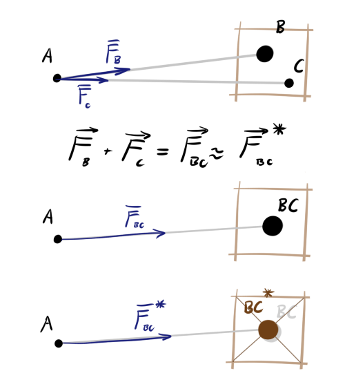
For simulations with such a huge number of bodies one has to go for some simplifications. Note that for the three bodies A, B and C, the sum of the forces acting on A from B and C is equal to the force that a single body (BC) would have if placed at the center of mass point of B and C. This alone is not enough for optimization, therefore one more trick. We divide the space into cells. If the distance from body A to the cell is large and there is more than one body in the cell, we will assume that an object with the total mass of objects inside is placed exactly in the center of this cell. Its position will deviate slightly from the present center of mass of the cell contents, but the farther the cell, the more insignificant will be the error in the angle of force.


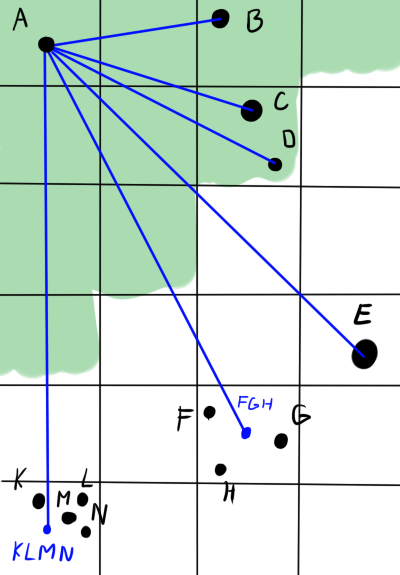
In the picture below, green indicates the area of ​​proximity of body A. Blue indicates the direction of action of the forces. The bodies B, C and D exert force on A separately. Although C and D are in the same cell, they are in the area of ​​accuracy. E also has power alone - it is one in a cage. But the objects F, G and H are far enough from A and close enough to each other, that the interaction can be brought closer. The center of the cell will not always coincide well with the real position of the center of gravity (see K, L, M, N), but on average, with a large distance and a large number of bodies, the error will be negligible.


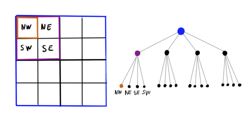
It became better: we reduced the effective number of objects several times. But how to choose the optimal size of the partition? If the partition is too small, there will be no sense from it, and if it is too large, the error will increase and you will have to set a very large distance at which we will be ready to sacrifice accuracy. Let's take another step forward: instead of a grid with a fixed step, we divide the plane's rectangle into a hierarchy of cells. Large cells contain small ones, even smaller ones, and so on. The resulting data structure is a tree, where each non-leaf node spawns four child nodes. This construction is called a quadtree . For the three-dimensional case, respectively, the octree (octotree) is used. Now, when calculating the force acting on a certain body, it is possible to bypass the tree until a cell with a sufficient level of fineness is encountered, after which an approximation is used.


Node that does not fall into any object makes no sense to shrink further, so this structure is not as heavy as it may seem at first glance. On the other hand, there is definitely an overhead, so I would say that as long as there are less than a hundred simulated objects, such a tricky data structure can be a bit harmful (depends on the implementation).

Now more formally:

Algorithm 1:
Let be $$$d$ - the distance from the body to the center of the considered cell, $$$s$ - the side of this cell, $$$\ theta$ - predetermined threshold of fineness. To determine the force exerted on an object $$$b$ , we bypass the quadtree, starting from the root.

1. If there is no element in the current cell, skip it.
2. Otherwise, if there is only one element in the node and it is not $$$b$ , directly add its effect to the total force
3. Otherwise, if $$$s / d \ leq \ theta$ , we consider this node as a single whole object, and add its total force, as described above.
4. Otherwise, we recursively run this procedure for all daughter cells of the current cell.

Here is a more detailed execution of the algorithm in steps. A beautiful animation of the Barnes-Hut galaxy simulation. Various implementations of Barnes-Hut can be found on the githab.

Obviously, such an interesting idea could not go unnoticed in other areas of science. Barnes-Hut is used wherever there are systems with a large number of objects, each of which acts on the others according to a simple law, which varies slightly in space: a swarm simulation, computer games. So the analysis of the data was no exception either. Let us write in more detail the stage of gradient descent (3) in t-SNE:

$$

$$\ frac {\ delta C} {\ delta y} = 4 \ sum_ {j \ neq i} {(p_ {ij} - q_ {ij}) q_ {ij} Z (y_i - y_j)}$$

$$

$$= 4 (\ sum_ {j \ neq i} {p_ {ij} q_ {ij} Z (y_i - y_j)} - \ sum_ {j \ neq i} {q_ {ij} ^ 2Z (y_i - y_j)) }$$

$$

$$= 4 (F_ {attr} + F_ {rep})$$

Where $$$F_ {attr}$ indicated attracting forces $$$F_ {req}$ - repulsive, and $$$Z$ - the normalizing factor. Thanks to previous optimization $$$F_ {attr}$ considered to be $$$O (uN)$ but $$$F_ {req}$ - yet $$$O (N ^ 2)$ . This is where the quadtree and Barens-Hut trick described above comes in handy, but instead of Newton's law $$$F = q_ {ij} ^ 2Z (y_i - y_j)$ . This simplification allows you to calculate $$$F_ {req}$ behind $$$O (N \ log {N})$ average. The disadvantage is obvious: errors due to the discretization of space. Laurens van der Maaten in the article above states that for the time being it is not even clear whether they are limited at all (there are links to relevant articles). Be that as it may, the results obtained with t-SNE Barens-Hut with normally matched $$$\ theta$ look wealthy and consistent. Usually you can put $$$\ theta = $ 0.2$ or $$$0.1$ and forget about it.

Is it even faster? Yes Why stop at the point-cell approximation, when you can simplify the situation even more: if two cells are far enough apart, you can bring more than just the final one $$$y$ , but also initial (cell-cell approximation). This is called the dual-tree algorithm (there is no Russian name yet). We do not run recursion above for each data instance, but begin to bypass the quadtree and when the fineness reaches the desired value, we begin to bypass the same quadtree and apply the total force from the second bypass cell to each instance inside the selected first bypass cell. This approach allows you to squeeze a little more speed, but the error starts to accumulate much faster, and you have to put less $$$\ theta$ . Yes, and implemented such a detour is not so much where.

LargeVis

Good, but is it even faster? Jian Tang and company, say yes!
Since we have already sacrificed accuracy, why not sacrifice determinism to the virgin . We will use random algorithms to get the result for $$$O (N)$ of time. First, instead of searching for the nearest neighbors using the vantage point tree, we use random projection trees (RT-trees). Secondly, instead of honestly calculating the gradient with simplifications through Barnes-Hut, we will simply sample the terms in the negative part $$$C (y)$ .

RT-trees

The idea of ​​splitting the plane using a quadtree was not bad. Now we will try to split the plane into sectors using something more simple. What about kd tree ?

Algorithm 2:
Options: $$$M$ - minimum size $$$X$ - data set
MakeTree ( $$$X$ )

1. If a $$$| X | \ leq M$ return current $$$X$ as a leaf node
2. Otherwise
   
   1. Randomly select the variable number $$$i \ in [0, d-1]$
   2. Rule (x): = $$$x_j \ leq$ median ( $$$z_ {i}: z_i \ in X$ ) // Predicate dividing the data subspace by a hyperplane perpendicular to the coordinate axis $$$i$ and passing through the median values $$$i$ -th variable of elements $$$X$ .
   3. LeftTree: = MakeTree ({x $$$\ in$ X: Rule (x) = true})
   4. RightTree: = MakeTree ({x $$$\ in$ X: Rule (x) = false})
   5. Redo [Rule, LeftTree, RightTree]

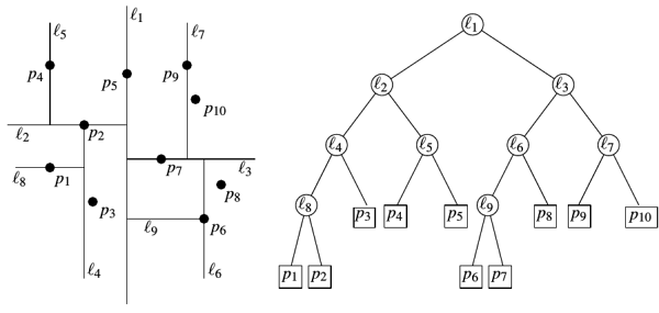
Somehow too primitive. The perpendicularity of the plane of splitting of some axis of coordinates looks suspicious. There is a more advanced version: random projection trees (RT-trees). We will recursively divide the space, each time choosing a random unit vector perpendicular to which the plane will go. For easy asymmetry of the tree, also add a little noise to the anchor point of the plane.

Algorithm 3:
ChooseRule (X) // Meta-function, which returns a predicate by which we will break the space

1. Choose a random unit vector from $$$v \ in \ mathcal {R} ^ d$
2. Choose random $$$y \ in X$
3. Let be $$$z \ in X$ - the furthest data point from it $$$X$
4. $$$\ delta$ : = random number in $$$[- 6 \ cdot \ left \ | y - z \ right \ | / \ sqrt {d}, 6 \ cdot \ left \ | y - z \ right \ | / \ sqrt {d}]$
5. Return Rule (x): = $$$x \ cdot v \ leq$ (median ( $$$z \ cdot v: z \ in X$ ) + $$$\ delta$ )

MakeRPTree ( $$$X$ )

1. If a $$$| X | \ leq M$ return current $$$X$ as a leaf node
2. Otherwise
   
   1. Rule (x): = ChooseRule (X)
   2. LeftTree: = MakeTree ({x $$$\ in$ X: Rule (x) = true})
   3. RightTree: = MakeTree ({x $$$\ in$ X: Rule (x) = false})
   4. Redo [Rule, LeftTree, RightTree]

Is such a rough and chaotic partition able to give at least some results? It turns out that yes! In the case when multidimensional data actually lie near a not very multidimensional hyperfolder, RT-trees behave quite decently (see the proofs on the first link here ). Even in the case when the data does indeed have an effective dimension comparable to $$$d$ , knowledge of projections carries a lot of information.

Hmm, complexity: calculate the median is still $$$O (| X |)$ and we do it on each of $$$O (\ log {N})$ steps. Simplify the choice of the hyperplane even more: in general, we abandon the anchor point. At each recursion step, we will simply choose two random points from the next $$$X$ and draw a plane equidistant from them.

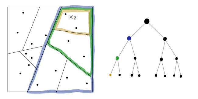
It seems that we have thrown out from the algorithm everything that at least somehow reminds of mathematical rigor or precision. How can the resulting trees help us find our closest neighbors? Obviously, the neighbors of the data points on the graph sheet are the first candidates for his kNN. But this is not certain: if the point lies next to the hyperplane of the partition, the real neighbors may be on a completely different sheet. The resulting approximation can be improved by building several RP-trees. The intersection of sheets of the resulting graphs for each $$$x$ is a much better area to look for.


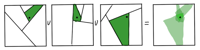
You don't need too many trees, it undermines the speed. The resulting approximation is brought to mind with the help of the heuristics of “the neighbor of my neighbor - most likely my neighbor”. It is argued that quite a few iterations are enough to get a decent result.



The authors of the article claim that the effective implementation of all this works for $$$O (N)$ of time. There is, however, one thing but they don’t mention: O-big swallows a gigantic constant, which is influenced $$$M$ , the number of RP-trees, and the number of stages of the heuristic adjustment.

Sampling

After calculating kNN, Jian Tang and KO consider the similarity of data in the original space using the same formula as in t-SNE.

$$

$$p_ {j | i} = \ frac {\ exp {(- \ left \ | x_i - x_j \ right \ | ^ 2 / (2 \ sigma ^ 2_i)}} {\ sum _ {(i, k) \ in Neigh} (\ exp {(- \ left \ | x_i - x_k \ right \ | / (2 \ sigma ^ 2_i)})}$$

$$

$$p_ {ij} = \ frac {p_ {j | i} + p_ {i | j}} {2}$$

Please note that the denominator amount is calculated only for kNN, the rest $$$p_ {j | i}$ equal to 0; also $$$p_ {ii} = 0$ .

After that, a clever theoretical maneuver is proposed: now we are looking at the resulting $$$w_ {ij} \ equiv p_ {ij}$ , as on the weights of edges of some graph, where nodes are elements $$$X$ . Encode information about the weights of this graph using a set of $$$y$ in display space. Let the probability of observing a binary unweighted edge $$$e_ {ij}$ equals

$$

$$P (\ exists e_ {ij}) = \ frac {1} {1 + \ left \ | y_k - y_m \ right \ |}$$

The t-distribution is again used, only slightly differently; still remember the different number of neighbors in different layers in spaces with different $$$d$ . The probability that the original graph had an edge with a weight in $$$w_ {ij}$ :

$$

$$P (\ exists w_ {ij}) = P (\ exists e_ {ij}) ^ {w_ {ij}}$$

Multiply the probabilities for all edges and get the location $$$y$ maximum likelihood method:

$$

$$O = \ prod _ {(i, j) \ in E} P (\ exists e_ {ij}) ^ {w_ {ij}} \ prod _ {(i, j) \ in \ vec {E}} (1 - P (\ exists e_ {ij}) ^ {\ gamma}$$

Where $$$\ vec {E}$ - the set of all pairs that are not included in the list of nearest neighbors, and $$$\ gamma$ - a hyperparameter showing the influence of non-existent edges. We logarithmically:

$$

$$\ log {O} \ propto \ sum _ {(i, j) \ in E} {w_ {ij} \ log {P (\ exists e_ {ij})}} + \ sum _ {(i, j) \ in \ vec {E}} {\ gamma \ log {(1 - P (\ exists e_ {ij}))}} \ rightarrow \ max$$

Again received a sum consisting of two parts: one attracts to each other $$$y$ close to each other $$$x$ the other pushes away $$$y$ , $$$x$ which were not neighbors of each other, they only look different. Again, we got the problem that the exact calculation of the second sub-volume will take $$$O {(N ^ 2)}$ , as there are a lot of missing arcs in our column. This time, instead of using a quadtree, it is proposed to sample the nodes of the graph, to which there are no arcs. This technique came from word processing. There for faster learning context for each word $$$j$ which is in the text next to the word $$$i$ , take not all the words from the dictionary, which are next to $$$i$ they do not occur, but only a few arbitrary words, with a probability proportional to 3/4 of the degree of their frequency (the 3/4 indicator is chosen empirically, more here ). We are for each node $$$j$ to which there is a rib from $$$i$ with weight in $$$w_ {ij}$ , we will sample several arbitrary nodes, to which there are no edges, in proportion to the 3/4 degree of the number of arcs emanating from those nodes.

$$

$$\ log {O} \ approx \ sum _ {(i, j) \ in E} {w_ {ij} (\ log {P (\ exists e_ {ij})}} + \ sum_ {k = 1} ^ M {E_ {j_k \ sim P_n (j)} \ gamma \ log {(1 - P (\ exists e_ {ij_k})))}} \ rightarrow \ max$$

Where $$$M$ - the number of negative edges per node, and $$$P_n (j) \ sim d_j ^ {3/4}$ .

Because $$$w_ {ij}$ can vary within rather wide limits; an advanced version of the sampling technique should be used to stabilize the gradient. Instead of fingering $$$j$ with the same frequency, we will take them by the probability proportional $$$w_ {ij}$ and pretend to be a single edge.

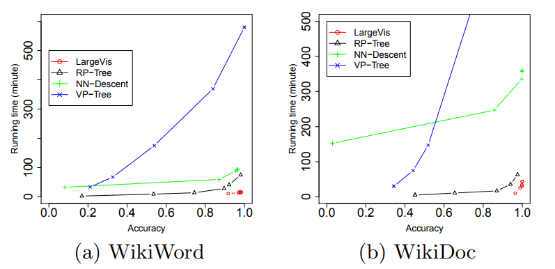
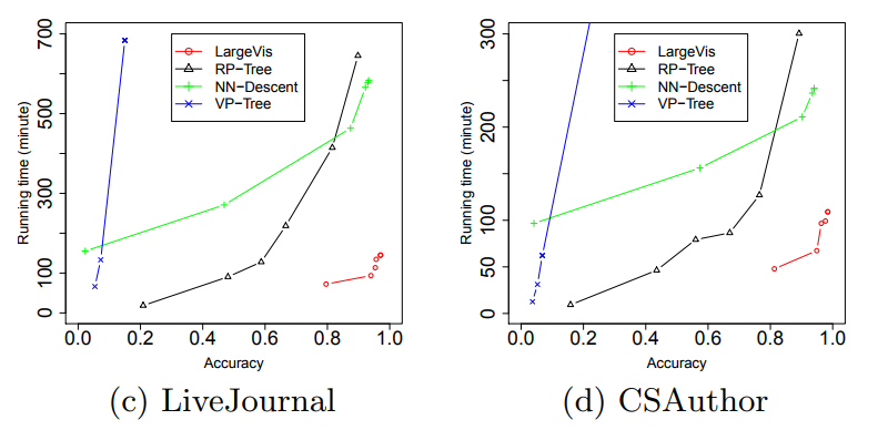
Wow What gives us all these tricks? Approximately fivefold increase in speed on moderately large datasets compared with Barnes-Hut t-SNE!






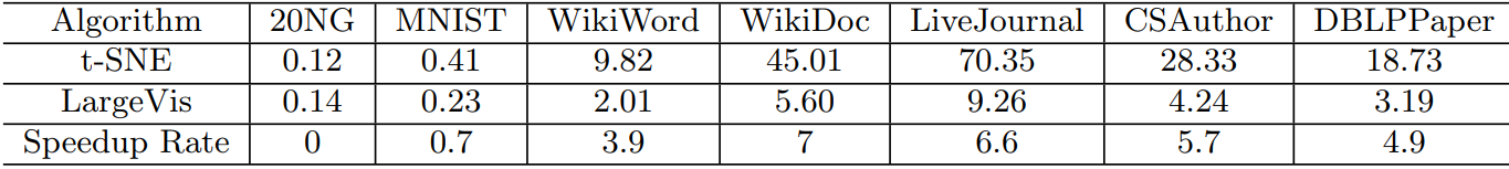
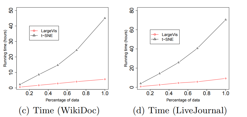
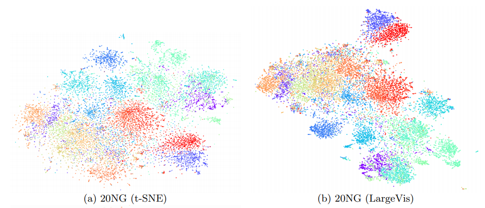
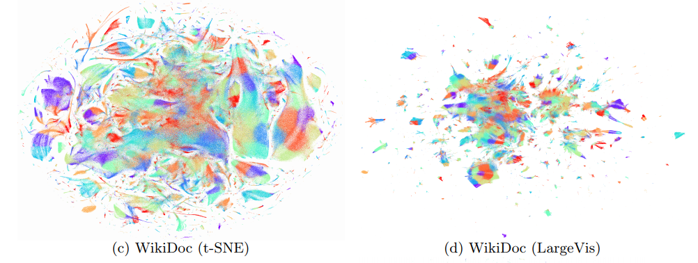
(Pictures taken from the article )

The quality of visualization is about the same. An attentive reader will notice that 20 Newsgroups ( $$| X | ≈ 20000 ) LargeVis loses t-SNE. This is the effect of the insidious constant, which remained behind the scenes. Students, remember, mindless use of algorithms with a lesser degree under the O-big hurts your health! Finally, a couple of practical moments. There is the officialimplementation ofLargeVis, but in my opinion the code is slightly ugly there, use at your own risk. Number of negative samples per node$| X | \approx 20000$

$$M is usually taken equal to 5 (came from computer word processing). Experiments have shown a very slight increase in quality while increasing$M$$$M from 3 to 7. The number of trees should be taken the larger, the larger the data set, but not too much. Focus on the minimum value of 10 for$M$$$| X | < 10 5 and close to the excess 100$|X| < 10^5$$$$|X| > 10^7$ . $$ g a m m a the creators of the algorithm take a value of 7, without explaining why. Most importantly: LargeVis perfectly parallel at all stages of work. Due to the sparseness of the weights matrix, asynchronous sparse gradient descent on different streams is unlikely to touch each other.$\ gamma$

Conclusion

Thanks for attention.I hope, now it has become clearer to you that this is the mysterious method = 'barnes_hut' and angle in the parameters of the sklearn'ovskogo TSNE, and you will not be lost when you need to visualize from ten million records. If you are working with a large amount of data, maybe you can find your own use of Barens-Hut or decide to implement LargeVis. Just in case, here are brief notes on the work of the latter. Have a nice day!