We already got acquainted with the PostgreSQL indexing mechanism and the access methods interface , and examined hash indexes , B-trees , GiST and SP-GiST indexes. And in this part we will deal with the GIN index.

GIN

- Gin? .. Gin - it seems to be such an American alcoholic drink? ..
- I am not a drink, oh an inquisitive lad! - the old man flared up again, he realized himself again and again took himself in hand. - I am not a drink, but a powerful and fearless spirit, and there is no such magic in the world that I could not do.

Lazar Lagin, "Old Man Hottabych."
')
Gin stands for indexed invert index and should be considered as a genie, not a drink.

README

General idea

GIN stands for Generalized Inverted Index - this is the so-called reverse index . It works with data types whose values ​​are not atomic, but consist of elements. In this case, not the values ​​themselves are indexed, but individual elements; each element refers to the values ​​in which it occurs.

A good analogy for this method is the alphabetical index at the end of the book, where for each term there is a list of pages where this term is mentioned. Like the pointer in the book, the index method should provide a quick search for indexed items. For this, they are stored in the form of a B-tree already familiar to us (another, simpler implementation is used for it, but in this case it is irrelevant). Each item has an ordered set of links to table rows containing values ​​with this item. The orderliness is not critical for sampling data (the sorting order of TIDs does not carry much sense), but it is important from the point of view of the internal structure of the index.


Items are never removed from the GIN index. It is believed that the values ​​containing the elements may disappear, appear, change, but the set of elements of which they consist is rather static. This solution greatly simplifies the algorithms that provide parallel operation with the index of several processes.

If the list of TIDs is small enough, it is placed in the same page as the item (and is called the posting list). But if the list is large, we need a more efficient data structure, and we already know it - this is again a B-tree. Such a tree is located in separate data pages (and is called a posting tree).

Thus, the GIN index consists of a B-tree of elements, to the leaf entries of which B-trees or flat lists of TIDs are attached.

Like the GiST and SP-GiST indexes discussed earlier, GIN provides an application developer with an interface to support various operations on complex data types.

Full text search

The main area of ​​application of the gin method is the acceleration of full-text search, so it is logical to consider this index in more detail using this example.

In the part about GiST, there was already a small introduction to full-text search, so we will not repeat and get right to the point. It is clear that complex values ​​in this case are documents, and elements of these documents are lexemes.

Take the same example that we looked at in the GiST part (just repeat the chorus twice):

postgres=# create table ts(doc text, doc_tsv tsvector);
CREATE TABLE
postgres=# insert into ts(doc) values
(' '), (' '),
(', , '), (', , '),
(' '), (' '),
(', , '), (', , '),
(' '), (' '),
(', , '), (', , ');
INSERT 0 12

postgres=# set default_text_search_config = russian;
SET
postgres=# update ts set doc_tsv = to_tsvector(doc);
UPDATE 12
postgres=# create index on ts using gin(doc_tsv);
CREATE INDEX

The possible structure of such an index is shown in the figure:



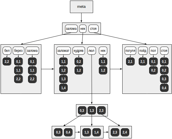
Unlike all previous illustrations, references to table lines (TIDs) are shown not by arrows, but by numeric values ​​on a dark background (page number and position on the page):

postgres=# select ctid, doc, doc_tsv from ts;
ctid | doc | doc_tsv
--------+-------------------------+--------------------------------
(0,1) | | '':3 '':2 '':4
(0,2) | | '':3 '':2 '':4
(0,3) | , , | '':1,2 '':3
(0,4) | , , | '':1,2 '':3
(1,1) | | '':2 '':3 '':1
(1,2) | | '':3 '':2 '':1
(1,3) | , , | '':3 '':1,2
(1,4) | , , | '':3 '':1,2
(2,1) | | '':3 '':2
(2,2) | | '':1 '':2 '':3
(2,3) | , , | '':3 '':1,2
(2,4) | , , | '':3 '':1,2
(12 rows)

In our speculative example, the list of TIDs fit into ordinary pages for all lexemes, except for "lyul." This token met in as many as six documents and for her the list of TIDs was placed in a separate B-tree.

How, by the way, to understand how many documents contain a token? For a small table, the “direct” method shown below will work, and we will see how to deal with large ones.

postgres=# select (unnest(doc_tsv)).lexeme, count(*) from ts group by 1 order by 2 desc;
lexeme | count
---------+-------
| 6
| 4
| 4
| 3
| 3
| 2
| 2
| 2
| 1
| 1
| 1
(11 rows)

We also note that, in contrast to a regular B-tree, the pages of the GIN index are not related to a bidirectional, but to a unidirectional list. This is sufficient, since a tree is always traversed in one direction only.

Request example

How will the following query be performed in our example?

postgres=# explain(costs off)
select doc from ts where doc_tsv @@ to_tsquery(' & ');
QUERY PLAN
------------------------------------------------------------------------
Bitmap Heap Scan on ts
Recheck Cond: (doc_tsv @@ to_tsquery(' & '::text))
-> Bitmap Index Scan on ts_doc_tsv_idx
Index Cond: (doc_tsv @@ to_tsquery(' & '::text))
(4 rows)

First, separate lexemes (search keys) are selected from the search query: “standing” and “curly”. This is done by a special API function that takes into account the data type and the strategy defined by the class of statements:

postgres=# select amop.amopopr::regoperator, amop.amopstrategy
from pg_opclass opc, pg_opfamily opf, pg_am am, pg_amop amop
where opc.opcname = 'tsvector_ops'
and opf.oid = opc.opcfamily
and am.oid = opf.opfmethod
and amop.amopfamily = opc.opcfamily
and am.amname = 'gin'
and amop.amoplefttype = opc.opcintype;
amopopr | amopstrategy
-----------------------+--------------
@@(tsvector,tsquery) | 1
@@@(tsvector,tsquery) | 2 @@ ( )
(2 rows)

Next, we find both keys in the B-tree of tokens and iterate over the ready lists of TIDs. We get:

• for “standing” - (0,1), (0,2), (0,3), (0,4);
• for “curly” - (0,2), (1,2).

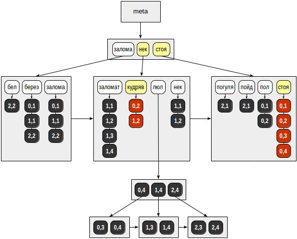
Finally, for each TID found, the API match function is called, which must determine which of the found strings match the search query. Since in our query, the tokens are combined with the logical “and”, a single string (0,2) is returned:

| | |
| | |
TID | | | &
-------+------+--------+-----------------
(0,1) | T | f | f
(0,2) | T | T | T
(0,3) | T | f | f
(0,4) | T | f | f
(1,2) | f | T | f

And we get the result:

postgres=# select doc from ts where doc_tsv @@ to_tsquery(' & ');
doc
-------------------------

(1 row)

If we compare this approach with the one we considered for GiST, the advantage of GIN for full-text search seems obvious. But not everything is so simple.

Slow update problem

The point is that inserting or updating data in a GIN index is relatively slow. Each document usually contains many tokens to be indexed. Therefore, when a single document appears or changes, it is necessary to make massive changes to the index tree.

On the other hand, if several documents change at once, then a part of the tokens may coincide with them, and the total amount of work will be less than if the documents are changed one by one.

The GIN index has a fastupdate storage parameter, which you can specify when creating the index or change it later:

postgres=# create index on ts using gin(doc_tsv) with (fastupdate = true);
CREATE INDEX

When enabled, changes will accumulate as a separate unordered list (in separate linked pages). When this list is large enough, or when performing a cleaning process, all accumulated changes are simultaneously made to the index. What is considered a “large enough” list is determined by the configuration parameter gin_pending_list_limit or by the same storage parameter of the index itself.

But this approach also has negative sides: first, the search slows down (due to the fact that besides the tree you have to look through an unordered list), and second, the next change can suddenly take a long time if the unordered list is overflowed.

Partial match search

Partial match can be used in full-text search. The request is formulated, for example, as follows:

gin=# select doc from ts where doc_tsv @@ to_tsquery(':*');
doc
-------------------------


, ,
, ,

, ,
, ,
(7 rows)

Such a request will find documents in which there are tokens starting with the “hall”. That is, in our example, “the crease” (which is obtained from the word “I hack”) and the “zalomat” (from the word “zaromati”).

The query, of course, will work in any case, even without indices, but the GIN allows you to speed up such a search:

postgres=# explain (costs off)
select doc from ts where doc_tsv @@ to_tsquery(':*');
QUERY PLAN
--------------------------------------------------------------
Bitmap Heap Scan on ts
Recheck Cond: (doc_tsv @@ to_tsquery(':*'::text))
-> Bitmap Index Scan on ts_doc_tsv_idx
Index Cond: (doc_tsv @@ to_tsquery(':*'::text))
(4 rows)

In this case, in the tree of tokens there are all tokens that have the prefix specified in the search query, and are combined with the logical “or”.

Frequent and rare lexemes

To see how the indexing works on real data, take the pgsql-hackers mailing list, which we have already used in the GiST topic. This version of the archive contains 356,125 letters with the date of departure, subject, author and text.

fts=# alter table mail_messages add column tsv tsvector;
ALTER TABLE
fts=# set default_text_search_config = default;
SET
fts=# update mail_messages
set tsv = to_tsvector(body_plain);
NOTICE: word is too long to be indexed
DETAIL: Words longer than 2047 characters are ignored.
...
UPDATE 356125
fts=# create index on mail_messages using gin(tsv);
CREATE INDEX

Take the lexeme, which is found in a large number of documents. A query using unnest will not work on such a volume of data, and the correct way is to use the ts_stat function, which gives information about tokens, the number of documents in which they are encountered, and the total number of entries.

fts=# select word, ndoc
from ts_stat('select tsv from mail_messages')
order by ndoc desc limit 3;
word | ndoc
-------+--------
re | 322141
wrote | 231174
use | 176917
(3 rows)

Choose "wrote".

And take some rare word in the list of developers, for example, "tattoo":

fts=# select word, ndoc from ts_stat('select tsv from mail_messages') where word = 'tattoo';
word | ndoc
--------+------
tattoo | 2
(1 row)

Are there any documents in which these tokens appear at the same time? It turns out there is:

fts=# select count(*) from mail_messages where tsv @@ to_tsquery('wrote & tattoo');
count
-------
1
(1 row)

The question is how to execute this query. If, as described above, to get lists of TIDs for both lexemes, the search will turn out to be obviously ineffective: we will have to iterate over more than two hundred thousand values, of which only one will be the result. Fortunately, using the statistics of the scheduler, the algorithm understands that the “token” lexeme is often found, and the “tattoo” is rare. Therefore, the search is performed on a rare lexeme, and the resulting two documents are then checked for the presence of the “wrote” token in them. As it can be seen - the request is executed quickly:

fts=# \timing on
Timing is on.

fts=# select count(*) from mail_messages where tsv @@ to_tsquery('wrote & tattoo');
count
-------
1
(1 row)
Time: 0,959 ms

Although the search simply “wrote” - significantly longer:

fts=# select count(*) from mail_messages where tsv @@ to_tsquery('wrote');
count
--------
231174
(1 row)
Time: 2875,543 ms (00:02,876)

Such optimization works, of course, not only for two tokens, but also in more complex cases.

Sample limit

The peculiarity of the gin access method is that the result is always returned in the form of a bitmap: this method does not know how to issue TIDs one by one. That is why all query plans that are encountered in this part use bitmap scan.

Therefore, limiting a sample by index using the LIMIT clause is not quite effective. Pay attention to the predicted cost of the operation (the “cost” field of the Limit node):

fts=# explain (costs off)
select * from mail_messages where tsv @@ to_tsquery('wrote') limit 1;
QUERY PLAN
-----------------------------------------------------------------------------------------
Limit (cost=1283.61..1285.13 rows=1)
-> Bitmap Heap Scan on mail_messages (cost=1283.61..209975.49 rows=137207)
Recheck Cond: (tsv @@ to_tsquery('wrote'::text))
-> Bitmap Index Scan on mail_messages_tsv_idx (cost=0.00..1249.30 rows=137207)
Index Cond: (tsv @@ to_tsquery('wrote'::text))
(5 rows)

The cost is estimated at 1283.61, which is slightly more than the cost of building the entire bitmap 1249.30 (the “cost” field of the Bitmap Index Scan node).

Therefore, the index has a special ability to limit the number of results. The threshold value is set in the gin_fuzzy_search_limit configuration parameter and defaults to zero (no limit occurs). However, it can be installed:

fts=# set gin_fuzzy_search_limit = 1000;
SET
fts=# select count(*) from mail_messages where tsv @@ to_tsquery('wrote');
count
-------
5746
(1 row)

fts=# set gin_fuzzy_search_limit = 10000;
SET
fts=# select count(*) from mail_messages where tsv @@ to_tsquery('wrote');
count
-------
14726
(1 row)

As you can see, the query produces a different number of rows for different values ​​of the parameter (if index access is used). The restriction is not precise; more lines than specified can be issued - therefore fuzzy.

Compact view

Among other things, GIN-indices are good for their compactness. Firstly, if the same token is found in several documents (as it usually happens), it is stored only once in the index. Secondly, TIDs are stored in an index in an orderly manner, and this makes it possible to use simple compression: each next one in the TID list is actually stored as the difference with the previous one — usually a small number that requires much less bits than a full 6 -byte TID.

To get some idea of ​​volume, create a B-tree in the text of the letters. Fair comparison, of course, does not work:

• GIN is built on a different data type (tsvector, not text), but it’s smaller,
• but the size of the letters for the B-tree has to be shortened to about two kilobytes.

But nonetheless:

fts=# create index mail_messages_btree on mail_messages(substring(body_plain for 2048));
CREATE INDEX

At the same time, we will build the GiST index:

fts=# create index mail_messages_gist on mail_messages using gist(tsv);
CREATE INDEX

The size of the index after complete cleaning (vacuum full):

fts=# select pg_size_pretty(pg_relation_size('mail_messages_tsv_idx')) as gin,
pg_size_pretty(pg_relation_size('mail_messages_gist')) as gist,
pg_size_pretty(pg_relation_size('mail_messages_btree')) as btree;
gin | gist | btree
--------+--------+--------
179 MB | 125 MB | 546 MB
(1 row)

Due to the compactness of the representation, the GIN index can be used to migrate from Oracle as a replacement for bitmap indexes (I won’t go into details, but for inquiring minds I’ll leave a link to Lewis' post ). As a rule, bitmap indexes are used for fields that have some unique values ​​— which is fine for GIN as well. And to build a bitmap, as we saw in the first part , PostgreSQL can on the fly based on any index, including the GIN.

GiST or GIN?

For many data types, there are classes of operators for both GiST and GIN, which raises the question: what to use? Perhaps, it is already possible to draw any conclusions.

As a rule, GIN gains in accuracy and speed of search from GiST. If the data does not change often, but you need to search quickly - most likely the choice will fall on the GIN.

On the other hand, if the data changes actively, the overhead of updating the GIN may be too large. In this case, you will have to compare both options and choose the one whose indicators will be better balanced.

Arrays

Another example of using the gin method is array indexing. In this case, the elements of the arrays fall into the index, which allows speeding up a series of operations on them:

postgres=# select amop.amopopr::regoperator, amop.amopstrategy
from pg_opclass opc, pg_opfamily opf, pg_am am, pg_amop amop
where opc.opcname = 'array_ops'
and opf.oid = opc.opcfamily
and am.oid = opf.opfmethod
and amop.amopfamily = opc.opcfamily
and am.amname = 'gin'
and amop.amoplefttype = opc.opcintype;
amopopr | amopstrategy
-----------------------+--------------
&&(anyarray,anyarray) | 1
@>(anyarray,anyarray) | 2
<@(anyarray,anyarray) | 3
=(anyarray,anyarray) | 4
(4 rows)

Our demo database has routes with flight information. Among other things, it contains the days_of_week column - an array of days of the week on which flights are made. For example, a flight from Vnukovo to Gelendzhik departs on Tuesdays, Thursdays and Sundays:

demo=# select departure_airport_name, arrival_airport_name, days_of_week
from routes
where flight_no = 'PG0049';
departure_airport_name | arrival_airport_name | days_of_week
------------------------+----------------------+--------------
| | {2,4,7}
(1 row)

To build the index, we “materialize” the view into the table:

demo=# create table routes_t as select * from routes;
SELECT 710
demo=# create index on routes_t using gin(days_of_week);
CREATE INDEX

Now, using the index, we can find out all flights departing on Tuesdays, Thursdays and Sundays:

demo=# explain (costs off) select * from routes_t where days_of_week = ARRAY[2,4,7];
QUERY PLAN
-----------------------------------------------------------
Bitmap Heap Scan on routes_t
Recheck Cond: (days_of_week = '{2,4,7}'::integer[])
-> Bitmap Index Scan on routes_t_days_of_week_idx
Index Cond: (days_of_week = '{2,4,7}'::integer[])
(4 rows)

It turns out, these 6 pieces:

demo=# select flight_no, departure_airport_name, arrival_airport_name, days_of_week from routes_t where days_of_week = ARRAY[2,4,7];
flight_no | departure_airport_name | arrival_airport_name | days_of_week
-----------+------------------------+----------------------+--------------
PG0005 | | | {2,4,7}
PG0049 | | | {2,4,7}
PG0113 | - | | {2,4,7}
PG0249 | | | {2,4,7}
PG0449 | | | {2,4,7}
PG0540 | | | {2,4,7}
(6 rows)

How is such a request? In the same way as described above:

1. From the search query, whose role is played by the array {2,4,7}, the elements (search keys) are distinguished. Obviously, these will be the values ​​"2", "4" and "7".
2. In the element tree there are selected keys and for each of them a list of TIDs is selected.
3. Of all the TIDs found, the consistency function selects those that fit the operator from the query. For operator = only those TIDs that are met in all three lists are suitable (in other words, the initial array must contain all the elements). But this is not enough: it is also necessary that the array does not contain any other values ​​— and we cannot check this condition by index. Therefore, in this case, the access method asks the indexing mechanism to double-check all the issued TIDs in the table.

It is interesting that there are strategies (for example, “contained in an array”) that cannot check anything at all and are forced to recheck all the TIDs found in the table.

But what if we need to find out flights departing on Tuesdays, Thursdays and Sundays from Moscow? The additional condition will not be supported by the index and will fall into the Filter column:

demo=# explain (costs off)
select * from routes_t where days_of_week = ARRAY[2,4,7] and departure_city = '';
QUERY PLAN
-----------------------------------------------------------
Bitmap Heap Scan on routes_t
Recheck Cond: (days_of_week = '{2,4,7}'::integer[])
Filter: (departure_city = ''::text)
-> Bitmap Index Scan on routes_t_days_of_week_idx
Index Cond: (days_of_week = '{2,4,7}'::integer[])
(5 rows)

In this case, it is not scary (the index already selects only 6 lines), but in cases where the additional condition increases the selectivity, I would like to have such an opportunity. True, just create an index does not work:

demo=# create index on routes_t using gin(days_of_week,departure_city);
ERROR: data type text has no default operator class for access method "gin"
HINT: You must specify an operator class for the index or define a default operator class for the data type.

But the btree_gin extension will help, adding classes of GIN operators that mimic the operation of a regular B-tree.

demo=# create extension btree_gin;
CREATE EXTENSION
demo=# create index on routes_t using gin(days_of_week,departure_city);
CREATE INDEX

demo=# explain (costs off)
select * from routes_t where days_of_week = ARRAY[2,4,7] and departure_city = '';
QUERY PLAN
---------------------------------------------------------------------
Bitmap Heap Scan on routes_t
Recheck Cond: ((days_of_week = '{2,4,7}'::integer[]) AND
(departure_city = ''::text))
-> Bitmap Index Scan on routes_t_days_of_week_departure_city_idx
Index Cond: ((days_of_week = '{2,4,7}'::integer[]) AND
(departure_city = ''::text))
(4 rows)


Jsonb

Another example of a complex data type for which there is built-in GIN support is JSON. To work with JSON values, a number of operators and functions are currently defined, some of which can be accelerated using indexes:

postgres=# select opc.opcname, amop.amopopr::regoperator, amop.amopstrategy as str
from pg_opclass opc, pg_opfamily opf, pg_am am, pg_amop amop
where opc.opcname in ('jsonb_ops','jsonb_path_ops')
and opf.oid = opc.opcfamily
and am.oid = opf.opfmethod
and amop.amopfamily = opc.opcfamily
and am.amname = 'gin'
and amop.amoplefttype = opc.opcintype;
opcname | amopopr | str
----------------+------------------+-----
jsonb_ops | ?(jsonb,text) | 9
jsonb_ops | ?|(jsonb,text[]) | 10 -
jsonb_ops | ?&(jsonb,text[]) | 11
jsonb_ops | @>(jsonb,jsonb) | 7 JSON-
jsonb_path_ops | @>(jsonb,jsonb) | 7
(5 rows)

There are, as you can see, two classes of operators: jsonb_ops and jsonb_path_ops.

The first class of operators, jsonb_ops, is used by default. All keys, values ​​and elements of arrays fall into the index as elements of the source JSON document. To each of them, a sign is added whether this element is a key (this is necessary for “exist” strategies that distinguish keys and values).

For example, imagine several lines from routes in the form of JSON as follows:

demo=# create table routes_jsonb as
select to_jsonb(t) route
from (
select departure_airport_name, arrival_airport_name, days_of_week
from routes
order by flight_no limit 4
) t;
SELECT 4
demo=# select ctid, jsonb_pretty(route) from routes_jsonb;
ctid | jsonb_pretty
-------+-----------------------------------------------
(0,1) | { +
| "days_of_week": [ +
| 1 +
| ], +
| "arrival_airport_name": "", +
| "departure_airport_name": "-" +
| }
(0,2) | { +
| "days_of_week": [ +
| 2 +
| ], +
| "arrival_airport_name": "-", +
| "departure_airport_name": "" +
| }
(0,3) | { +
| "days_of_week": [ +
| 1, +
| 4 +
| ], +
| "arrival_airport_name": "", +
| "departure_airport_name": "-"+
| }
(0,4) | { +
| "days_of_week": [ +
| 2, +
| 5 +
| ], +
| "arrival_airport_name": "-", +
| "departure_airport_name": "" +
| }
(4 rows)

demo=# create index on routes_jsonb using gin(route);
CREATE INDEX

The index may have the following form:



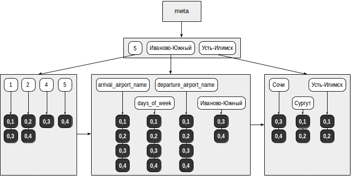
Now, for example, such a query can be executed using an index:

demo=# explain (costs off)
select jsonb_pretty(route)
from routes_jsonb
where route @> '{"days_of_week": [5]}';
QUERY PLAN
---------------------------------------------------------------
Bitmap Heap Scan on routes_jsonb
Recheck Cond: (route @> '{"days_of_week": [5]}'::jsonb)
-> Bitmap Index Scan on routes_jsonb_route_idx
Index Cond: (route @> '{"days_of_week": [5]}'::jsonb)
(4 rows)

The @> operator checks whether the specified path is present ( "days_of_week": [5] ), starting from the root of the JSON document. In our case, the query returns one line:

demo=# select jsonb_pretty(route) from routes_jsonb where route @> '{"days_of_week": [5]}';
jsonb_pretty
----------------------------------------------
{ +
"days_of_week": [ +
2, +
5 +
], +
"arrival_airport_name": "-",+
"departure_airport_name": "" +
}
(1 row)

The query is executed as follows:

1. From the search query ( "days_of_week": [5] ), elements (search keys) are highlighted: "days_of_week" and "5".
2. In the tree of elements there are selected keys and for each of them a list of TIDs is selected: for “5” - (0.4) and for “days_of_week” - (0.1), (0.2), (0.3) , (0.4).
3. Of all the TIDs found, the consistency function selects those that fit the operator from the query. For the @> operator, documents that do not contain all the elements from the search query are definitely not suitable, so only (0.4) remains. But the remaining TID must be rechecked against the table, because the index does not understand the order in which the found elements are found in the JSON document.

More information about other operators can be read in the documentation .

In addition to regular operations for working with JSON, the jsquery extension has been around for a long time, defining a query language with richer capabilities (and, of course, with support for GIN indices). And in 2016, the new SQL standard came out, which defines its own set of operations and the SQL / JSON path query language. The implementation of this standard has already been completed and we hope it will appear in PostgreSQL 11.

Inside

You can look inside the GIN index using the pageinspect extension.

fts=# create extension pageinspect;
CREATE EXTENSION

Information from the metastpage shows general statistics:

fts=# select * from gin_metapage_info(get_raw_page('mail_messages_tsv_idx',0));
-[ RECORD 1 ]----+-----------
pending_head | 4294967295
pending_tail | 4294967295
tail_free_size | 0
n_pending_pages | 0
n_pending_tuples | 0
n_total_pages | 22968
n_entry_pages | 13751
n_data_pages | 9216
n_entries | 1423598
version | 2

The structure of the page provides a special area, “opaque” (opaque) for ordinary programs like cleaning (vacuum), in which access methods can store their information. This data for the GIN is shown in the gin_page_opaque_info function. For example, you can find out the composition of the index pages:

fts=# select flags, count(*)
from generate_series(1,22967) as g(id), -- n_total_pages
gin_page_opaque_info(get_raw_page('mail_messages_tsv_idx',g.id))
group by flags;
flags | count
------------------------+-------
{meta} | 1
{} | 133 B-
{leaf} | 13618 B-
{data} | 1497 B- TID-
{data,leaf,compressed} | 7719 B- TID-
(5 rows)

The gin_leafpage_items function returns information about TIDs stored in {data, leaf, compressed} pages:

fts=# select * from gin_leafpage_items(get_raw_page('mail_messages_tsv_idx',2672));
-[ RECORD 1 ]---------------------------------------------------------------------
first_tid | (239,44)
nbytes | 248
tids | {"(239,44)","(239,47)","(239,48)","(239,50)","(239,52)","(240,3)",...
-[ RECORD 2 ]---------------------------------------------------------------------
first_tid | (247,40)
nbytes | 248
tids | {"(247,40)","(247,41)","(247,44)","(247,45)","(247,46)","(248,2)",...
...

Here you can see that the leaf pages of the TID tree actually do not contain separate pointers to table rows, but small compressed lists.

Properties

Let's look at the properties of the gin access method (the queries were cited earlier ):

amname | name | pg_indexam_has_property
--------+---------------+-------------------------
gin | can_order | f
gin | can_unique | f
gin | can_multi_col | t
gin | can_exclude | f

Interestingly, the GIN supports the creation of multi-column indexes. At the same time, unlike the usual B-tree, not composite keys will be stored in it, but still separate elements, but only with indication of the column number.

Index properties:

name | pg_index_has_property
---------------+-----------------------
clusterable | f
index_scan | f
bitmap_scan | t
backward_scan | f

Please note that one-by-one (index scan) results are not supported, only bitmap scan is possible.

Backward scan is not supported: this feature is relevant only for index scanning, but not for scanning on a bitmap.

And column level properties:

name | pg_index_column_has_property
--------------------+------------------------------
asc | f
desc | f
nulls_first | f
nulls_last | f
orderable | f
distance_orderable | f
returnable | f
search_array | f
search_nulls | f

Nothing is available here: neither sorting (which is understandable), nor using an index as a cover (the document itself is not stored in the index), nor working with undefined values ​​(does not make sense for elements of a complex type).

Other data types

Here are some more extensions that add GIN support for some data types.

• pg_trgm allows you to determine the "similarity" of words by comparing the number of matching sequences of three letters (trigrams). Two classes of operators are added, gist_trgm_ops and gin_trgm_ops, supporting different operators, including comparison using LIKE and regular expressions. This extension can be used in conjunction with full-text search in order to offer word variations for typos.
  
• hstore implements key-value storage. For this data type, there are classes of operators for different access methods, including GIN. Although, with the advent of the jsonb data type, there are no particular reasons to use hstore.
  
• intarray extends the functionality of integer arrays. Index support includes both GiST and GIN (operator class gin__int_ops).
  

And two extensions have already been mentioned in the text:

• btree_gin adds GIN support for common data types to use in a multi-column index along with complex types.
  
• jsquery defines the query language for JSON and the class of operators for its index support. This extension is not included in the standard PostgreSQL distribution.
  

Continued .