A short course of machine learning or how to create a neural network to solve the scoring problem
We often hear such verbal constructions as “machine learning”, “neural networks”. These expressions are already tightly embedded in the public consciousness and are most often associated with pattern and speech recognition, with the generation of human-like text. In fact, machine learning algorithms can solve many different types of problems, including helping small businesses, online publishing, and anything. In this article I will explain how to create a neural network that is able to solve the real business problem of creating a scoring model. We will consider all the stages: from data preparation to creating a model and assessing its quality.
Questions that are discussed in the article:
')
• How to collect and prepare data for building a model?
• What is a neural network and how is it arranged?
• How to write your neural network from scratch?
• How to properly train a neural network based on available data?
• How to interpret the model and its results?
• How to correctly assess the quality of the model?
"The question of whether a computer can think is no more interesting,
than the question of whether a submarine can swim. "
Edsger Vibe Dijkstra
In many companies, sales managers communicate with potential customers, give them demonstrations, talk about the product. They give, so to speak, their soul for the hundredth time to be torn apart by those who may have fallen into their hands completely by accident. Often, customers do not understand enough what they need, or what the product can give them. Communicating with such clients brings neither pleasure nor profit. And the most unpleasant thing is that due to time constraints, you can not pay enough attention to a really important client and miss the deal.
I am a software mathematician in the Serpstat seo analytics service. Recently, I received an interesting task to improve the scoring model that already exists and works with us, re-evaluating the factors that influence the success of the sale. Scoring was considered based on the survey of our clients, and each item, depending on the answer to the question, contributed a certain number of points to the total score. All these points for different questions were placed on the basis of statistical hypotheses. The scoring model was used, as time went on, the data was collected and one day came to me. Now that I had a sufficient sample, I could safely build hypotheses using machine learning algorithms.
I will tell you how we built our scoring model. This is a real case with real data, with all the difficulties and limitations that we encountered in a real business. So, first things first.
We will dwell on all stages of work:
▸ Data collection
▸ Preprocessing
▸ Building a model
▸ Quality analysis and model interpretation
Consider the design, creation and training of a neural network. I describe all this, solving a real scoring problem, and constantly reinforce a new theory with an example.
Data collection
First you need to understand what questions will represent the client (or just an object) in the future model. We approach the task seriously, since on its basis a further process is built. First, it is necessary not to miss the important signs that describe the object, and second, to create stringent criteria for deciding on a sign. Based on experience, I can distinguish three categories of questions:
- Booleans (bicategorial), the answer to which is: Yes or No (1 or 0). For example, the answer to the question: does the client have an account?
- Categorical, the answer to which is a specific class. Usually there are more than two classes (multi-categorical), otherwise the question can be reduced to a Boolean one. For example, color: red, green or blue.
- Quantitative, the answers to which are the numbers characterizing a specific measure. For example, the number of hits per month: fifteen.
Why do I dwell on it in such detail? Usually, when considering a classical problem solved by machine learning algorithms, we deal only with numerical data. For example, the recognition of black and white handwritten numbers from the image of 20 by 20 pixels. In this example, 400 numbers (describing the brightness of a black and white pixel) represent one example from a sample. In general, the data need not be numeric. The fact is that when building a model, you need to understand what types of questions the algorithm can deal with. For example: a decision tree is trained on all types of questions, and a neural network accepts only numerical input data and is trained only on quantitative attributes. Does this mean that we have to give up some questions for the sake of a better model? Not at all, just need to properly prepare the data.
The data should have the following classical structure: feature vector for each i-th client X (i) = {x (i) 1 , x (i) 2 , ..., x (i) n } and the class Y (i) - category showing whether he bought or not. For example: client (3) = {green, bitter, 4.14, yes} - bought.
Based on the above, we will try to provide a data format with types of questions for further preparation:
| class: (category) | Colour: (category) | taste: (category) | weight: (number) | solid: (bool) |
|---|---|---|---|---|
| - | red | sour | 4.23 | Yes |
| - | green | bitter | 3.15 | not |
| + | green | bitter | 4.14 | Yes |
| + | blue | sweet | 4.38 | not |
| - | green | salty | 3.62 | not |
Table 1 - Example of training sample data before preprocessing
Preprocessing
Once the data is collected, they need to be prepared. This stage is called preprocessing. The main task of preprocessing is to display data in a format suitable for learning the model. There are three main manipulations with data at the preprocessing stage:
- Creating a vector feature space where the examples of the training sample will live. In essence, this is the process of bringing all the data into numerical form. This saves us from categorical, Boolean and other non-numeric types.
- Data normalization. The process by which we achieve, for example, that the average value of each attribute for all data is zero, and the variance is single. Here is the most classic example of data normalization: X = (X - μ) / σnormalization function
def normalize(X): return (XX.mean())/X.std() - Changing the dimension of the vector space. If the vector space of features is too large (millions of features) or small (less than ten), then you can apply methods to increase or decrease the dimension of space:
- To increase the dimension, you can use part of the training sample as reference points , adding the distance to these points in the feature vector. This method often leads to the fact that in spaces of higher dimensionality the sets become linearly separable, and this simplifies the task of classification.
- To reduce the dimension most often use PCA. The main objective of the principal component method is the search for new linear combinations of features along which the dispersion of the values of the projections of the elements of the training sample is maximized.
One of the most important tricks in constructing a vector space is the method of representation as a number of categorical and boolean types. Meet: One-Hot (Rus. Unitary Code). The main idea of such a coding is to represent a categorical feature as a vector in a vector space with a dimension corresponding to the number of possible categories. The value of the coordinates of this category is taken as one, and all other coordinates are reset. With boolean values, everything is quite simple, they turn into real units or zeros.
For example, the sampling element can be either bitter, or sweet, or salty, or sour, or umami (meat). Then the One-Hot encoding will be the following: bitter = (1, 0, 0, 0, 0), sweet = (0, 1, 0, 0, 0), salty = (0, 0, 1, 0, 0), acid = (0, 0, 0, 1, 0), umami = (0, 0, 0, 0, 1). If you have a question why there are five tastes, not four, then read this article about the taste sensory system , well, this has nothing to do with scoring, and we will use four, confining ourselves to the old classification.
Now we have learned to turn categorical signs into ordinary numerical vectors, and this is very useful. After all the manipulations on the data, we get a training sample that is suitable for any model. In our case, after applying the unitary encoding and normalization, the data looks like this:
| class: | red: | green: | blue: | bitter: | sweet: | salti: | sour: | weight: | solid: |
|---|---|---|---|---|---|---|---|---|---|
| 0 | one | 0 | 0 | 0 | 0 | 0 | one | 0.23 | one |
| 0 | 0 | one | 0 | one | 0 | 0 | 0 | -0.85 | 0 |
| one | 0 | one | 0 | one | 0 | 0 | 0 | 0.14 | one |
| one | 0 | 0 | one | 0 | one | 0 | 0 | 0.38 | 0 |
| 0 | 0 | one | 0 | 0 | 0 | one | 0 | -0.48 | 0 |
Table 2 - Example of training sample data after preprocessing
It can be said that preprocessing is the process of mapping the data that we understand to a less convenient form for a person, but to a favorite form.
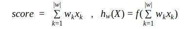
The scoring formula most often represents the following linear model:

Where, k is the question number in the questionnaire, w k is the coefficient of the contribution of the answer to this k-th question to the total scoring, | w | - the number of questions (or coefficients), x k - the answer to this question. At the same time, questions can be any, as we have discussed: boolean (yes or no, 1 or 0), numerical (for example, height = 175) or categorical, but presented in the form of a unitary encoding (green from the list: red, green or blue = [0, 1, 0]). At the same time, we can assume that categorical questions break down into as many Boolean ones as there are categories in the response options (for example: client red? Client green? Client blue?).
Model selection
Now the most important: the choice of the model. Today, there are many machine learning algorithms on the basis of which you can build a scoring model: Decision Tree (decision tree), KNN (k-nearest neighbors method), SVM (support vector method), NN (neural network). And the choice of model should be based on what we want from it. First, how much the decisions that influenced the model results should be understandable. In other words, how important it is for us to be able to interpret the structure of the model.
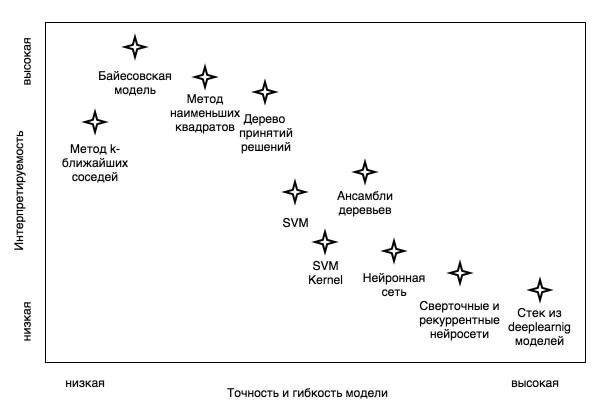
Fig. 1 - Dependence of machine learning algorithm flexibility and interpretability of the resulting model
In addition, not all models are easy to build, some require very specific skills and very, very powerful hardware. But the most important thing is the implementation of the constructed model. It happens that the business process is already established, and the introduction of a complex model is simply impossible. Or a linear model is required, in which customers, when answering questions, receive positive or negative points depending on the answer option. Sometimes, on the contrary, there is the possibility of implementation, and even requires a complex model that takes into account very unobvious combinations of input parameters, which finds the relationship between them. So, what to choose?
In choosing a machine learning algorithm, we stopped at a neural network. Why? First, there are now many cool frameworks, such as TensorFlow, Theano. They make it possible to very deeply and seriously customize the architecture and parameters of training. Secondly, the ability to change the device model from a single-layer neural network, which, by the way, is well interpreted, to a multi-layer one, which has an excellent ability to find non-linear dependencies, changing only a couple of lines of code. In addition, a trained single-layer neural network can be turned into a classic additive scoring model that adds points for answers to various survey questions, but more on that later.
Now a little theory. If for you such things as neuron, activation function, loss function, gradient descent and the method of back propagation of error are native words, then you can safely skip it all. If not, welcome to the short course of artificial neural networks.
Short course of artificial neural networks
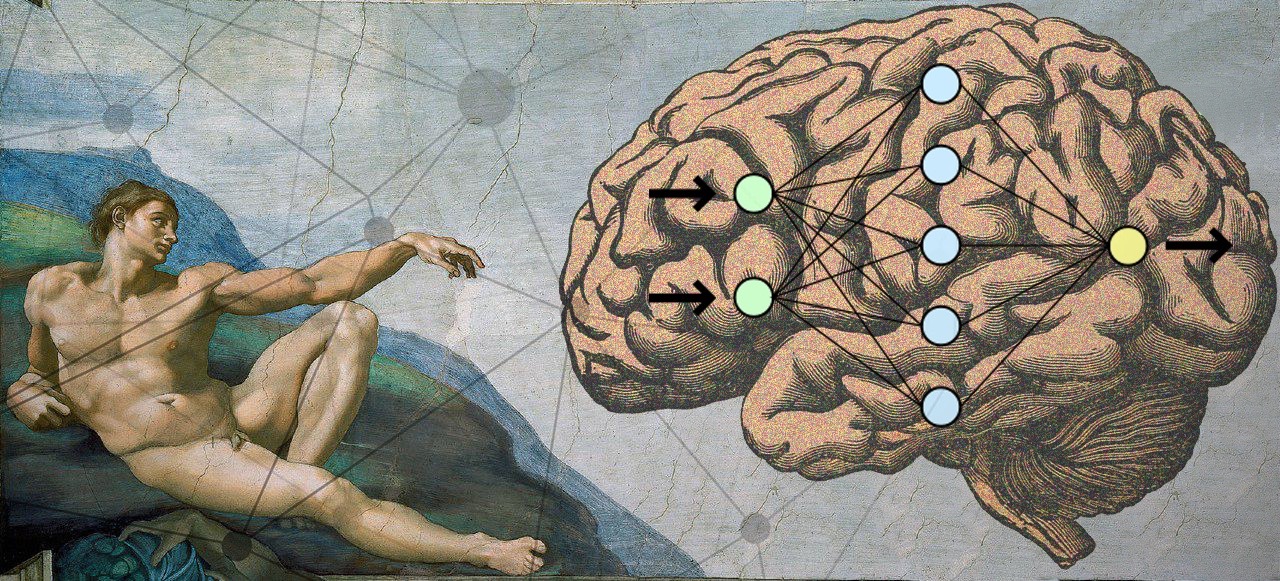
To begin with, artificial neural networks (ANN) are mathematical models of the organization of real biological neural networks (BNS). But unlike mathematical models of BNS, the ANN does not require an exact description of all chemical and physical processes, such as the description of the “ignition” of the action potential (AP), the work of neurotransmitters, ion channels, secondary mediators, transporter proteins, and others. the work of real BNS only at a functional, not at the physical level.
The basic element of a neural network is a neuron. Let's try to make the simplest functional mathematical model of a neuron. To do this, we describe in general terms the functioning of a biological neuron.
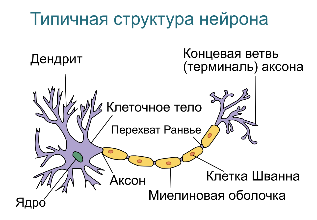
Fig. 2 - Typical structure of a biological neuron
As we can see, the structure of a biological neuron can be simplified to the following: dendrites, the body of the neuron and axon. Dendrites are branching processes that collect information from the entrance to a neuron (this may be external information from receptors, for example, from a cone in the case of color or internal information from another neuron). In that case, if the incoming information activated a neuron (in the biological case, the potential became higher than some threshold), an excitation wave (PD) is generated, which propagates through the neuron's body membrane, and then through the axon, by emitting a neurotransmitter, transmits a signal to other nerve cells. cells or tissues.
Based on this, Warren McCulloch and Walter Pitts in 1943 proposed a model of a mathematical neuron. And in 1958, Frank Rosenblatt, based on the McCulloch-Pitts neuron, created a computer program, and then a physical device, the perceptron. This is how the history of artificial neural networks began. Now consider the structural model of the neuron, with which we will deal further.

Fig. 3 - The model of the mathematical neuron McCullock-Pitts
Where:
- X is the input vector of parameters. Vector (column) of numbers (biol. Degree of activation of different receptors), which came to the input of the neuron.
W is the weights vector (in the general case, the weights matrix), numerical values that change in the learning process (biol. Training based on synaptic plasticity, the neuron learns to respond correctly to signals from its receptors). - Adder is a functional block of a neuron that adds all input parameters multiplied by their respective weights.
- The activation function of the neuron is the dependence of the value of the output of the neuron on the value coming from the adder.
- The following neurons, where the value from the output of the given neuron is fed to one of the set of their own inputs (this layer may be absent if this neuron is the last, terminal).
math neuron implementation
import numpy as np def neuron(x, w): z = np.dot(w, x) output = activation(z) return output Then classical artificial neural networks are assembled from these minimal structural units. The following terminology has been adopted:
- The input (receptor) layer is a vector of parameters (features). This layer does not consist of neurons. We can say that this is digital information, taken by receptors from the "external" world. In our case, this is customer information. The layer contains as many elements as the input parameters (plus the bias-term needed to shift the activation threshold).
- An associative (hidden) layer is a deep structure capable of memorizing examples, finding complex correlations and non-linear dependencies, and building abstractions and generalizations. In general, this is not even a layer, but a multitude of layers between input and output. It can be said that each layer prepares a new (higher-level) feature vector for the next layer. This layer is responsible for the appearance in the learning process of high-level abstractions. The structure contains as many neurons and layers as you please, and may even be absent (in the case of the classification of linearly separable sets).
- The output layer is a layer, each neuron of which is responsible for a specific class. The output of this layer can be interpreted as a function of the probability distribution of the belonging of an object to different classes. A layer contains as many neurons as there are classes in the training set. If there are two classes, then you can use two output neurons or limit it to just one. In this case, one neuron is still responsible only for one class, but if it gives values close to zero, then the element of the sample according to its logic should belong to another class.
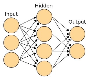
Fig. 4 - Classical neural network topology, with input (receptor), output, class-making, and associative (hidden) layer
Due to the presence of hidden associative layers, an artificial neural network is able to build hypotheses based on finding complex dependencies. For example, for convolutional neural networks that recognize images, the brightness values of the pixels of the image will be fed to the input layer, and the output layer will contain neurons responsible for specific classes (human, machine, tree, house, etc.). “Receptors” of hidden layers will start “by themselves” to appear (specialize) neurons, excited from straight lines, different inclination, then reacting to angles, squares, circles, primitive patterns: alternating stripes, geometric mesh patterns nty Closer to the output layers are neurons that react, for example, to the eye, the wheel, the nose, the wing, the leaf, the face, etc.
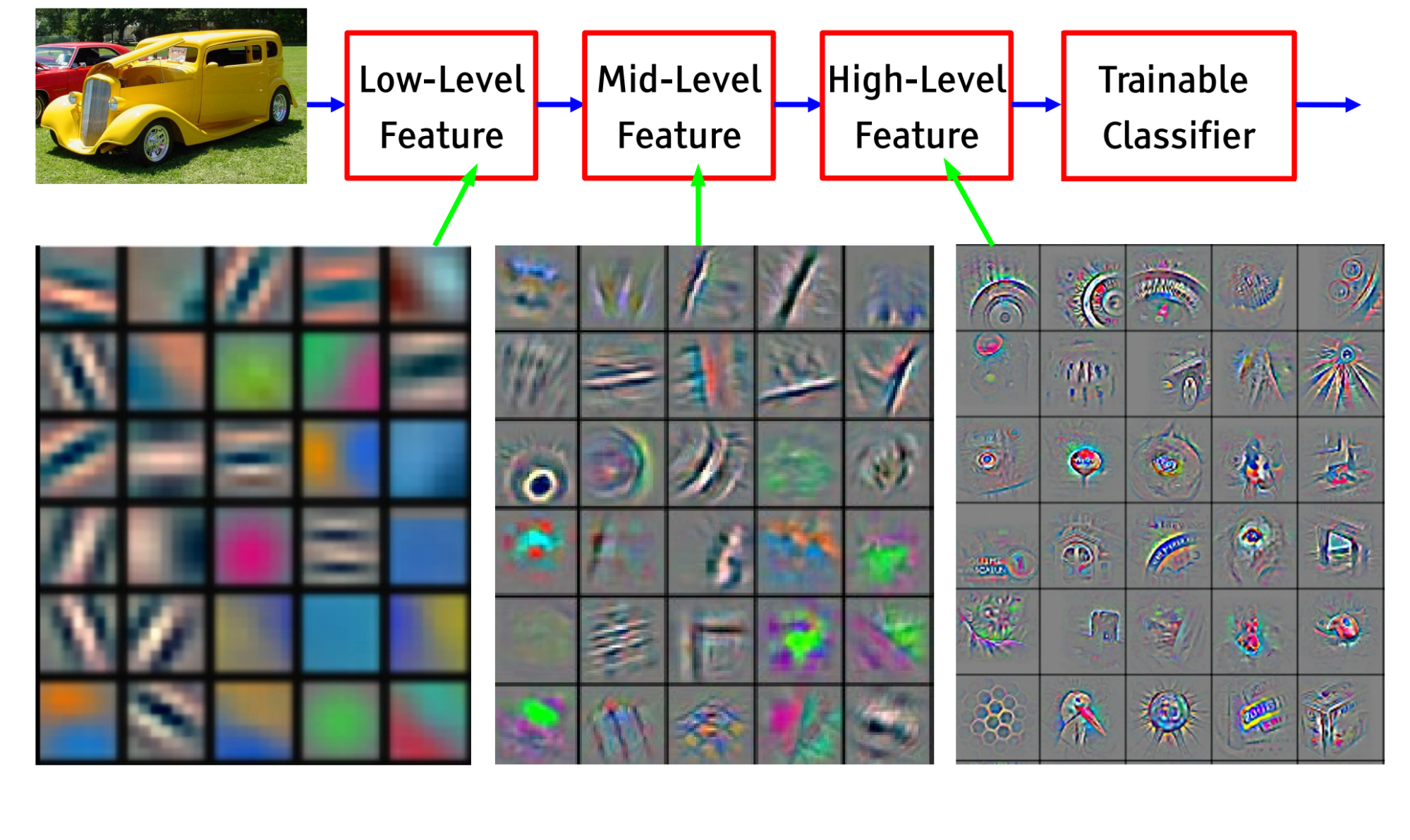
Fig. 5 - The formation of hierarchical associations in the process of learning convolutional neural network
Conducting a biological analogy, I would like to refer to the words of the remarkable neurophysiologist Vyacheslav Albertovich Dubynin concerning the speech model:
“Our brain is able to create, generate words that summarize the words of a lower level. Say, bunny, ball, cubes, doll - toys; toys, clothes, furniture are objects; and objects, houses, people are objects of the environment. And so a little more, and we get to abstract philosophical concepts, mathematical, physical. That is, speech generalization is a very important property of our associative parietal cortex, and it, in addition, is multi-layered and allows the speech model of the external world to form as integrity. At some point, it turns out that nerve impulses are able to move very actively along this speech model, and we call this movement the proud word “thinking”.
Lots of theory ?! But there is good news: in the simplest case, the entire neural network can be represented by a single neuron! Moreover, even one neuron often copes well with a task, especially when it comes to recognizing the class of an object in space in which the objects of these classes are linearly separable. Often, linear separability can be achieved by increasing the dimension of space, as described above, and be limited to just one neuron. But sometimes it is easier to add a couple of hidden layers to a neural network and not require a linear separability from the sample.
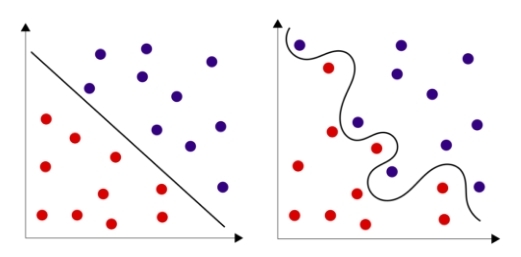
Fig. 6 - Linearly separable sets and linearly non-separable sets
Well, now let's describe all this formally. At the input of the neuron we have a vector of parameters. In our case, these are the results of the customer survey presented in the numerical form X (i) = {x (i) 1 , x (i) 2 , ..., x (i) n }. In addition, each client is assigned a Y (i) class, which characterizes the success of the lead (1 or 0). The neural network, in fact, must find the optimal separating hypersurface in the vector space, the dimension of which corresponds to the number of features. Learning a neural network in this case is finding such values (coefficients) of the matrix of weights W for which the neuron responsible for the class will produce values close to one in those cases if the customer buys and values close to zero if not.

As can be seen from the formula, the result of the neuron's work is the activation function (often denoted by) of the sum of the product of the input parameters and the coefficients sought in the learning process. Let us understand what is the activation function.
Since any real values can be input to a neural network, and the coefficients of the weights matrix can also be anything, and the result of the sum of their products can be any real number from minus to plus infinity. Each element of the training set has a class value relative to this neuron (zero or one). It is desirable to obtain a value from the neuron in the same range from zero to one, and decide on the class, depending on what this value is closer to. It is even better to interpret this value as the probability that an element belongs to this class. So, we need such a monotone smooth function that will display elements from the set of real numbers in the range from zero to one. The so-called sigmoid is great for this position.
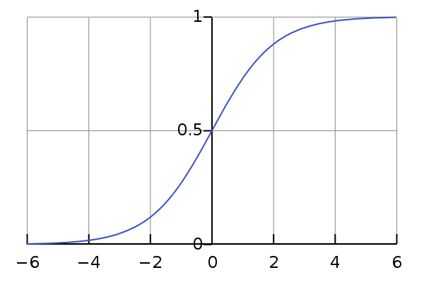
Fig. 7 - Logistic curve graph, one of the most classical representatives of the class sigmoid
activation function
def activation(z): return 1/(1+np.exp(-z)) By the way, in real biological neurons such a continuous activation function was not realized. In our cells with you there is a potential of rest, which averages -70mV. If information is sent to the neuron, then the activated receptor opens ion channels connected with it, which leads to an increase or decrease in potential in the cell. It is possible to draw an analogy between the strength of the reaction to the activation of the receptor and that obtained in the learning process with a single coefficient of the weight matrix. As soon as the potential reaches a value of -50mV, PD occurs, and the excitation wave travels along an axon to the presynaptic ending, throwing the neurotransmitter into the inter-synaptic medium. That is, the real biological activation is stepwise, not smooth: the neuron is either activated or not. This shows how mathematically we are free to build our models. Taking from nature the basic principle of distributed computing and learning, we are able to build a computational graph consisting of elements with any desired properties. In our example, we want to get continuous, rather than discrete values from the neuron. Although in the general case, the activation function may be different.
Here is the most important thing to extract from what was written above: “Neural network training (synaptic training) should be reduced to an optimal selection of weights matrix coefficients in order to minimize the allowed error.” In the case of a single-layer neural network, these coefficients can be interpreted as the contribution of element parameters to the probability of belonging to a specific class.
The result of the work of a neural network is called a hypothesis (English hypothesis). Denote by h (X), showing the dependence of the hypothesis on the input characteristics (parameters) of the object. Why a hypothesis? So historically. Personally, I like this term. As a result, we want the hypotheses of the neural network to correspond to reality as much as possible (real classes of objects). Actually here the basic idea of learning by experience is born. Now we need a measure describing the quality of the neural network. This functionality is usually called the "loss function" (born loss function). The functional is usually denoted by J (W), showing its dependence on the coefficients of the weights matrix. The less functionality, the less often our neural network is mistaken and the better it is. It is to minimize this functionality and learning is reduced. Depending on the coefficients of the weights matrix, the neural network may have different accuracy. The learning process is a movement along the loss functional hypersurface, the purpose of which is to minimize this functional.
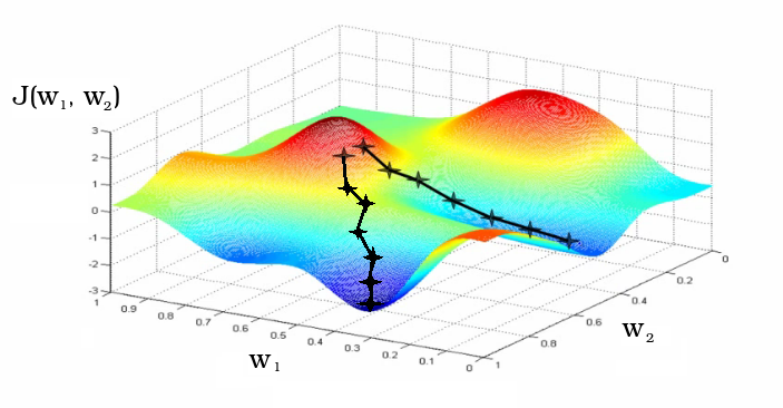
Fig. 8 - The learning process, as a gradient descent to the local minimum of the loss functional
Usually the weights matrix coefficients are initialized randomly. In the process of learning, the coefficients change. The graph shows two different iterative learning paths as a change in the coefficients w 1 and w 2 of the matrix of weights of the neural network initialized in the neighborhood.
, . , : () . . — , . , . . , .
: — , — , « » — ( , ). . () , :
- ( ) -1 1. , , . P — population or parents.
import random def generate_population(p, w_size): population = [] for i in range(p): model = [] for j in range(w_size + 1): # +1 for b (bias term) model.append(2 * random.random() - 1) # random initialization from -1 to 1 for b and w population.append(model) return np.array(population) - . , - , () . : , -0.1 0.1.
def mutation(genom, t=0.5, m=0.1): mutant = [] for gen in genom: if random.random() <= t: gen += m*(2*random.random() -1) mutant.append(gen) return mutant - , , ( — , — ). .
def accuracy(X, Y, model): A = 0 m = len(Y) for i, y in enumerate(Y): A += (1/m)*(y*(1 if neuron(X[i], model) >= 0.5 else 0)+(1-y)*(0 if neuron(X[i], model) >= 0.5 else 1)) return A - « » P . 2, . : 80%.
def selection(offspring, population): offspring.sort() population = [kid[1] for kid in offspring[:len(population)]] return population
def evolution(population, X_in, Y, number_of_generations, children): for i in range(number_of_generations): X = [[1]+[v.tolist()] for v in X_in] offspring = [] for genom in population: for j in range(children): child = mutation(genom) child_loss = 1 - accuracy(X_in, Y, child) # or child_loss = binary_crossentropy(X, Y, child) is better offspring.append([child_loss, child]) population = selection(offspring, population) return population . , -, τ — μ — . τ, ( -0.1 0.1) μ. .
, , , , , . . , . .
:
« — , — . , , — . , . , .»
, . , . , , , , , . , .
, . , , , — . , , , . , , , .
, , , , , , , .
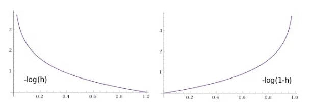
Fig. 9 — , : 1) ( ), 2) ( )
. , Y i- m , , .

, , (. cross entropy). C , .
def binary_crossentropy(X, Y, model): # loss function J = 0 m = len(Y) for i, y in enumerate(Y): J += -(1/m)*(y*np.log(neuron(X[i], model))+(1.-y)*np.log(1.-neuron(X[i], model))) return J , , , - , . , , , . — . , . () , () . , :

. -, , α ( ), . , , W, , , , .
def gradient_descent(model, X_in, Y, number_of_iteratons=500, learning_rate=0.1): X = [[1]+[v.tolist()] for v in X_in] m = len(Y) for it in range(number_of_iteratons): new_model = [] for j, w in enumerate(model): error = 0 for i, x in enumerate(X): error += (1/m) * (neuron(X[i], model) - Y[i]) * X[i][j] w_new = w - learning_rate * error new_model.append(w_new) model = new_model model_loss = binary_crossentropy(X, Y, model) return model . . . , , .
, — . , , 50%.
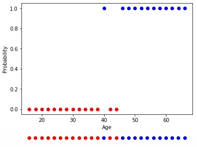
Fig. 10 —
, , . , bias , ( ). , , , - , ( — ), 42 .
0.5 42 , 0.5 . , 0.5 0.5 — . , - . , , x, .
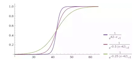
Fig. 11 — «» ,
, bias-term . f(x) , 42, 42 f(x-42). , , 0.25, f(0.25(x-24)). , :

w = 0.25, b = -10.5. , b (w 0 =b) , (x 0 =1). , «» 45 , x (15) = {x (15) 0 , x (15) 1 } = [1, 30], 68%. « ». , , . (w 0 =b w 1 ).
1 —
, . , .
2 —
. . «», . , «» .
3 —
, «»” .
4 —
:
- x;
- , a;
- , bias b;
- , w;
- h w,b (x) — .
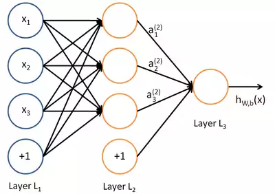
Fig. 12 —
TensorFlow . , . «», ( bias, bias ). , , () . .
5 —
, , . , . .
6 —
, , . , () . , .
7 —
. , . — . . () .
— , .
8 — « »
. « », . , . ReLU (rectified linear unit) , ( softmax -) .
, , , . , , .
Model training
, , . , . 5%, — 95%. ? 95% , , .
, , , . «» , .
, 20,000 1,000 , 500 . . , .
, : , 70% , 30% , .
, . :
- TP (True Positive) — . , , .
- FP (False Positive) — . , , . . , , , — - .
- FN (False Negative) — . , , ( ). . , .
- TN (True Negative) — . , , .
, (. precision) (. recall), .
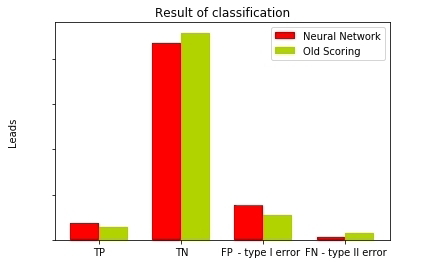
Fig. 13 —
, -, . , . .
— (. Accuracy). , . , , .

(. precision) , . , , 115, 37, 0.33. (. recall) . , 37, 43. 0.88.
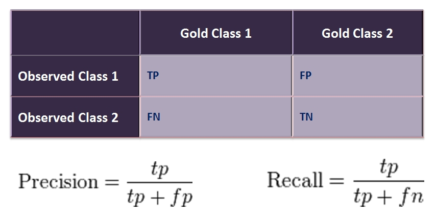
Fig. 14 — confusion matrix
F-
F- (. F1 score) — . , .

, .
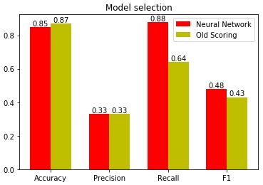
Fig. 15 —
, (. recall). 88% , 12%. 36% , 64%. , . , , .
, , , . () , , , . , .
( ):
, , , . , «» , . .
. , ( — ) 0.5 ( ). . . , .
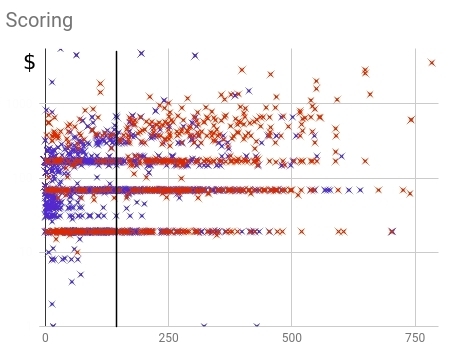
Fig. 16 — () ()
, . ( ) 64%.
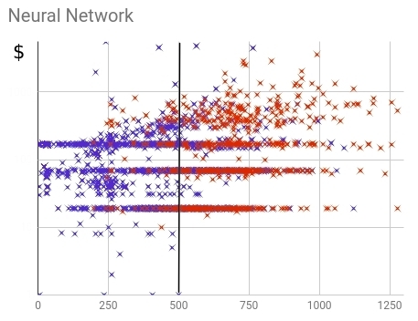
Fig. 17 — () ()
, . , , , — . ( ) 88%.
Result
, . , , , , .
, .
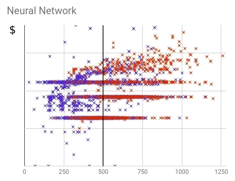
Fig. 18 — () ()
, , 87% . : 77%. , 10% . : 23% 24% . , .
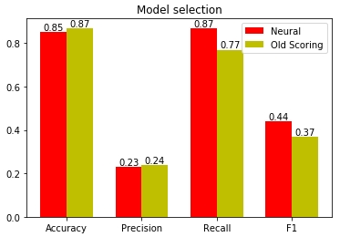
Fig. 19 —
, :
- data-mining.
- , .
- .
- .
- .
- , -.
, , .
Source: https://habr.com/ru/post/340792/
All Articles