Determination of the stability of automatic control systems for industrial robots

Introduction

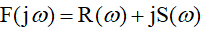
A necessary condition for the performance of the automatic control system (ACS) is its stability. Stability is commonly understood as the property of a system to restore the state of equilibrium, from which it was derived under the influence of perturbing factors after the cessation of their effect [1].

Formulation of the problem

Obtaining a simple, visual and accessible tool for solving problems of calculating the stability of automatic control systems, which is a prerequisite for the operation of any industrial robot and manipulator.

Theory is simple and brief

The stability analysis of the system according to Mikhailov’s method is reduced to the construction of the characteristic polynomial of a closed system (the denominator of the transfer function), a complex frequency function (characteristic vector):

(one)
')
Where

and

- respectively, the real and imaginary parts of the denominator of the transfer function, by the form of which one can judge the stability of the system.

Closed SAU is stable if the complex frequency function

starting on
the arrows are the origin of coordinates, passing successively n quadrants, where n is the order of the characteristic equation of the system, i.e.

(2)

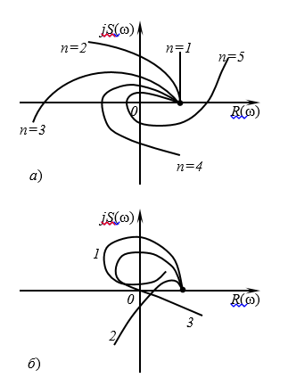
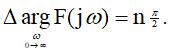
Figure 1. Amplitude-phase characteristics (hodographs) of the Mikhailov criterion: a) a stable system; b) - unstable system (1, 2) and systems on the stability boundary (3)

ACS by electric drive of industrial robot arm (MPR)

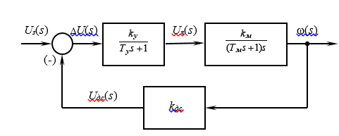
Figure 2 - Structural scheme of ACS electric drive MPR

The transfer function of this ACS has the following expression [2]:

(3)
where ky is the gain of the amplifier, km is the proportionality factor of the engine rotational frequency to the armature voltage, Tu is the electromagnetic time constant of the amplifier, Tm is the electromechanical time constant of the engine taking into account the load inertia (in its dynamic characteristics, the engine is a transfer function of the inertial and integrating links), cdc - proportionality coefficient between input and output values of the speed sensor, K - amplification factor Nia main circuit:

.

The numerical values in the transfer function expression are as follows:

K = 100 deg / (B ∙ s); kds = 0.01 V / (deg s); Ty = 0.01 s; Tm = 0.1 s.

Next, we write the characteristic polynomial of a closed system

replacing s with

(four)

Python solution

It should be noted here that no one has yet solved such problems in Python, in any case I have not found it. This was due to the limited possibilities of working with complex numbers. With the advent of SymPy, you can do the following:

from sympy import * T1,T2,w =symbols('T1 T2 w',real=True) z=factor ((T1*w*I+1)*(T2*w*I+1)*w*I+1) print ("    -\n%s"%z)

Where I is the imaginary unit, w is the circular frequency, T1 = T = 0.01, T2 = Tm = 0.1
We obtain an expanded expression for the polynomial:

Characteristic polynomial of a closed system -
-I * T1 * T2 * w ** 3 - T1 * w ** 2 - T2 * w ** 2 + I * w + 1

We immediately see that the polynomial is of the third degree. Now we get the imaginary and real parts in the symbolic display:

 zr=re(z) zm=im(z) print("  Re= %s"%zr) print("  Im= %s"%zm)

We get:

The real part Re = -T1 * w ** 2 - T2 * w ** 2 + 1
Imaginary part Im = -T1 * T2 * w ** 3 + w

We immediately see the second degree of the real part and the third imaginary part. Prepare the data for the construction of the Mikhailov hodograph. We introduce numerical values for T1 and T2, and we will change the frequency from 0 to 100 in increments of 0.1 and plot the graph:

 from numpy import arange import matplotlib.pyplot as plt x=[zr.subs({T1:0.01,T2:0.1,w:q}) for q in arange(0,100,0.1)] y=[zm.subs({T1:0.01,T2:0.1,w:q}) for q in arange(0,100,0.1)] plt.plot(x, y) plt.grid(True) plt.show()

From the graph is not visible, then the hodograph begins on a real positive axis. Need to change the scale of the axes. I will give a full listing of the program:

 from sympy import * from numpy import arange import matplotlib.pyplot as plt T1,T2,w =symbols('T1 T2 w',real=True) z=factor((T1*w*I+1)*(T2*w*I+1)*w*I+1) print("    -\n%s"%z) zr=re(z) zm=im(z) print("  Re= %s"%zr) print("  Im= %s"%zm) x=[zr.subs({T1:0.01,T2:0.1,w:q}) for q in arange(0,100,0.1)] y=[zm.subs({T1:0.01,T2:0.1,w:q}) for q in arange(0,100,0.1)] plt.axis([-150.0, 10.0, -15.0, 15.0]) plt.plot(x, y) plt.grid(True) plt.show()

We get:

The characteristic polynomial of a closed system - -I * T1 * T2 * w ** 3 - T1 * w ** 2 - T2 * w ** 2 + I * w + 1
The real part Re = -T1 * w ** 2 - T2 * w ** 2 + 1
Imaginary part Im = -T1 * T2 * w ** 3 + w

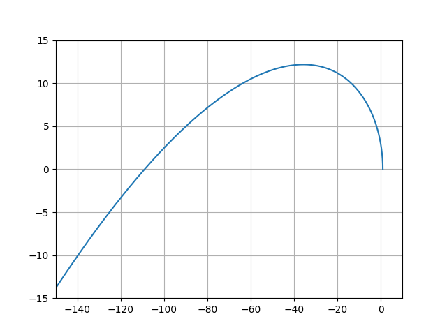
Now you can see that the hodograph begins on a real positive axis. The ACS is stable, n = 3, the hodograph coincides with that shown in the first figure.

Additionally, make sure that the hodograph begins on the real axis by adding the program with the following code for w = 0:

 print("  (%s,%s)"%(zr.subs({T1:0.01,T2:0.1,w:0}),zm.subs({T1:0.01,T2:0.1,w:0})))

We get:

Starting point M (1.0)

SAU welding robot

The tip of the welding unit (LLL) is brought to different places of the car body, quickly and accurately performs the necessary actions. It is required to determine the stability by the Mikhailov SAU criterion by positioning the NSO.

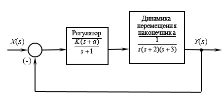
Figure 3. The block diagram of the ACS by positioning the NSO

The characteristic equation of this ACS will look like [1]:

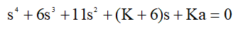
where K is the variable system gain, a is a definite positive constant. Numerical values: K = 40; a = 0.525.

Next, by replacing s with

, we get the Mikhailov function: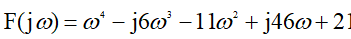

(five)

Python solution

 rom sympy import * from numpy import arange import matplotlib.pyplot as plt w =symbols(' w',real=True) z=w**4-I*6*w**3-11*w**2+I*46*w+21 print("    -\n%s"%z) zr=re(z) zm=im(z) print("  (%s,%s)"%(zr.subs({w:0}),zm.subs({w:0}))) print("  Re= %s"%zr) print("  Im= %s"%zm) x=[zr.subs({w:q}) for q in arange(0,100,0.1)] y=[zm.subs({w:q}) for q in arange(0,100,0.1)] plt.axis([-10.0, 10.0, -50.0, 50.0]) plt.plot(x, y) plt.grid(True) plt.show()

We get:

The characteristic polynomial of a closed system - w ** 4 - 6 * I * w ** 3 - 11 * w ** 2 + 46 * I * w + 21
Starting point M (21.0)
Real part Re = w ** 4 - 11 * w ** 2 + 21
Imaginary part Im = -6 * w ** 3 + 46 * w

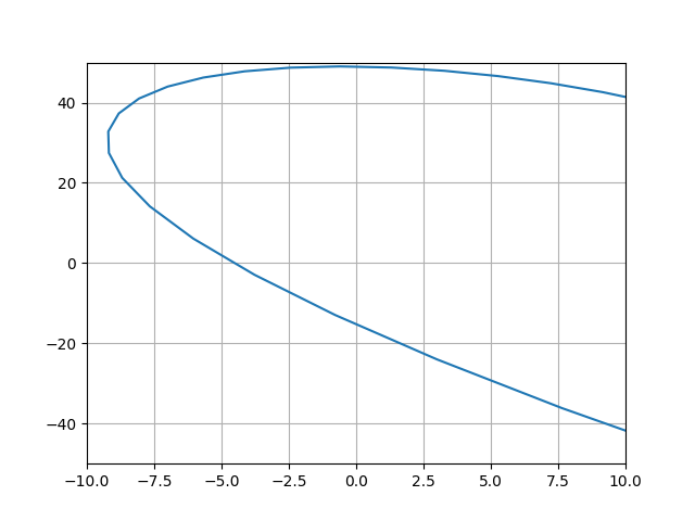
The built Mikhailov locus, starting at the real positive axis (M (21.0)), bends in the positive direction the origin of coordinates, passing successively four quadrants, which corresponds to the order of the characteristic equation. So, this ACS by positioning the NSO is stable.

findings

With the help of the SymPy Python module, a simple and visual tool was obtained for solving the problems of calculating the stability of automatic control systems, which is a prerequisite for the operation of any industrial robot and manipulator.

Determination of the stability of automatic control systems for industrial robots

Introduction

Formulation of the problem

Theory is simple and brief

ACS by electric drive of industrial robot arm (MPR)

Python solution

SAU welding robot

Python solution

findings

Links

More articles: