Non-Standard Clustering 5: Growing Neural Gas
Part One - Affinity Propagation
Part Two - DBSCAN
Part Three - Time Series Clustering
Part Four - Self-Organizing Maps (SOM)
Part Five - Growing Neural Gas (GNG)
Good day, Habr! Today I would like to talk about one interesting, but extremely little-known algorithm for the selection of clusters of atypical forms - Growing Neural Gas (GNG). Especially there is little information about this tool for analyzing data in runet: an article in Wikipedia , a story on Habré about a heavily modified version of GNG and a couple of articles with just a listing of the steps of the algorithm — that’s probably all. It is very strange, because few analyzers are able to work with time-varying distributions and normally perceive clusters of an exotic form - and this is precisely the strengths of GNG. Under the cut, I will try to explain this algorithm first with human language using a simple example, and then more strictly, in detail. I ask under the cat, if intrigued.
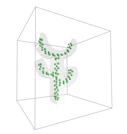
(In the picture: neural gas gently touches the cactus)
The article is organized as follows:
In addition, in the next article I plan to talk about several modifications and extensions of neural gas. If you want to grab onto the essence right away, you can skip the first section. If the second part seems too confusing, do not worry: the third part will be explained
Two programmer friends Alice and Boris decided to organize an emergency computer help agency. A lot of customers are expected, so during working hours they are sitting in their own car with all the equipment and waiting for calls. They do not want to pay for the focal point, so they quickly wrote a phone application that determines the client’s GPS location and directs the nearest car to it (for simplicity, suppose that when the order is not sent by the closest master, the machine returns almost right away). Also, Alice and Boris have radios to communicate with each other. However, they have only an approximate awareness of where to expect orders, and therefore, only an approximate understanding of where parking to expect new customers so that the way to them is as short as possible. Therefore, after each order, they slightly change their location and advise each other what area to capture. That is, if another client appeared 5 kilometers north and 1 kilometer east of Alisa’s current parking lot, and Alice was closest to him, then after the order she would move her parking lot 500 meters north and 100 meters east and advise Boris to move 50 meters to the north ( and 10 meters to the east, if it is not difficult).
')
Friends are going uphill, but they are still not satisfied with the time spent on empty travel to customers, so they include Vasilisa in her company so that she can take some of the orders from the dead zone to herself. Since Alice and Boris have not yet learned how to predict in advance where orders will come from, they offer Vasilisa to take a position between them and also adjust it. Vasilisa is given a walkie-talkie and two old members of the team take turns teaching her.
The question is whether to keep the dedicated radio Alice - Boris. They decide to decide on this later. If it turns out that Vasilisa is greatly displaced from the AB line and Alice will often become the second closest master for Boris's clients (and vice versa), then they will lead. No so no.
After some time, George joins the team. He is offered a place between people who most often and most of all have to change parking, since it is there that the most overhead costs. The default position is now reviewed only by the master, who is closest to the order and people who have direct access to the radio: if at some point the company has AB, BV, BD, and Boris accepts the order, then after the performance, Boris greatly changes his location, Vasilisa and Georgy - a little, Alice stands at the same parking lot, where she stood.
Sooner or later, the distribution of orders in the city begins to change: in some places all possible problems have already been healed and prevented. Already, an overgrown company does not take any special measures to deal with it, but simply continues to follow the parking adjustment algorithm. It works for some time, but at some point in time it turns out that most people in the Vasilisa area have learned to correct their problems themselves, and it never turns out to be either the first nearest master, or even the second. Walkie-talkie Vasilisa is silent, she is idle and can not change the dislocation. Alice and Boris think, and offer her a week to rest, after which to join between people who have too many orders.
After some time, the distribution of agency members in the city begins to approximate the distribution of people in need of assistance.
Okay, now for a more rigorous explanation. Expanding neural gas is a descendant of Kohonen self-organizing maps , an adaptive algorithm aimed not at finding a given fixed number of clusters, but at estimating the density of data distribution. Neurons are introduced into the data space in a special way, which adjust the location in the course of the algorithm. After the end of the cycle, it turns out that in places where the data density is high, there are too many neurons and they are connected with each other, and where small - one or two or none at all.
In the example above, Alice, Boris, Vasilisa and George play the role of GNG nodes, and their clients play the role of data samples.
Neuron gas does not use the data stationarity hypothesis. If instead of a fixed array of data X you have a function f(t) By sampling the data from some distribution that changes over time, GNG will easily work on it. In the course of the article, for simplicity, I will assume by default that the input is given pre-set X or not changing the distribution f(t) (and that these cases are equivalent, which is not entirely true). Moments relating to the case of varying distribution are considered separately.
We agree on the notation. Let be vecx - sample data dimension d , W - matrix with positions of neurons of size not larger than beta timesd where beta - a hyperparameter showing the maximum number of neurons (real size W may change during the operation of the algorithm). error - vector of size not larger than beta . Additional hyperparameters affecting the behavior of the algorithm: etawinner, etaneighbor - learning speed of the winning neuron and its neighbors, respectively, amax - the maximum age of communication between neurons, lambda - the period between iterations of generation of new neurons, alpha - the rate of attenuation of accumulated errors when creating new neurons, gamma - error attenuation every iteration, E - the number of epochs.
Algorithm 1:
Entrance: X, alpha, beta, gamma, etawinner, etaneighbor, lambda,amax,E,w1,w2
How many hyper parameters?
AT W initially 2 neurons w1 and w2 , they are connected by arc with age 0
error initialized with zeros
To the convergence to carry out:
Calm, now we shall understand.
The algorithm looks a bit ominous due to the abundance of items and parameters. Let's try to sort it out in parts.
If an array of data was supplied to the input of the algorithm X , we will assume that each neuron is a “prototype” of data, which in some way personifies them. Neurons create a Voronoi diagram in the data space and predict the average value of the data instances in each cell.
The picture shows an example of a simple Voronoi diagram: the plane is divided into sections corresponding to points inside. The set inside each colored polygon is closer to the central point of this polygon than to other black points.
There is an important difference in the coverage of the GNG distribution of neurons: each section of the plane above has the same “price”. This is not the case for neural gas: zones with a high probability of occurrence x have more weight:
(The red neuron covers a smaller area because there are more data instances on it)
The errors accumulated at the stage (3) errori show how good neurons are in this. If a neuron frequently and heavily updates the weight, then either it doesn’t fit the data well, or it covers too much of the distribution. In this case, it is worth adding one more neuron so that it takes a part of the updates on itself and reduces the global discrepancy to the data. This can be done in different ways (why not just poke it next to the neuron with the maximum error?), But if we still consider the errors of each neuron, then why not apply some heuristics? See (9.1), (9.2) and (9.3).
Since the data is sent to the loop randomly, the error is a statistical measure, but as long as there are far fewer neurons than the data (and usually it is), it is quite reliable.
In the figure below, the first neuron approximates data well, its error will increase slowly. The second neuron badly approximates data because it is far away from them; it will move and accumulate an error. The third node badly approximates data, because it grabs off a distribution zone where there are several clusters, and not just one. It will not move (on average), but will accumulate an error, and sooner or later will generate a child node.

Pay attention to paragraph (9.5) of the algorithm. It should already be clear to you: the new neuron takes part of the data from its brethren under its wing u and v . As a rule, we do not want to insert new nodes several times in the same place, so that we reduce the error in u and v and give them time to move to a new center. Also do not forget about point (10). First, we do not want errors to increase indefinitely. Secondly, we prefer the new errors to the old ones: if the node, while traveling to the data, has accumulated a big mistake, after which it has fallen into the place where it is well approximating the data, then it makes sense to unload it a little so that it does not share in vain.
Let's look at the scale weighting stage (4). Unlike gradient trigger algorithms (such as neural networks), which update everything at every step of the learning cycle, but little by little, neural gas and other SOM-like techniques concentrate on large-scale updating of weights only closest to vecx node and their direct neighbors. This is the strategy of Winner Takes All (WTA, the winner gets everything). This approach allows you to quickly find quite good w even with poor initialization, neurons receive large updates and quickly “reach” to the nearest data points. In addition, this way of updating gives the meaning of the accumulated errors. error .
If you remember how self-organizing cards work, you can easily understand where your ears grow from the idea of connecting nodes with edges (6). A priori information is transmitted to the SOM, as neurons should be located relative to each other. GNG does not have such initial data, they are searched on the fly. The goal, in part, is the same - to stabilize the algorithm, to make the distribution of neurons smoother, but more importantly, the constructed grid tells us exactly where to insert the next neuron and which neurons to delete. In addition, the resulting connection graph is invaluable at the stage of visualization.
Now a little more about the destruction of neurons. As mentioned above, by adding a node, we add a new “prototype” for the data. Obviously, some kind of restriction is needed on their number: although the increase in the number of prototypes is good from the point of view of data compliance, this is bad from the point of view of the benefits of clustering / visualization. What is the use of splitting, where there are exactly as many clusters as data points? Therefore, in GNG there are several ways to control their population. The first, the simplest - just a hard limit on the number of neurons (9). Sooner or later we stop adding nodes, and they can only shift to reduce the global error. Softer, the second - removal of neurons that are not associated with any other neurons (7) - (8). In this way, the old, outdated neurons, which correspond to the outliers, are removed, where the distribution has "disappeared" from, or that were generated in the first cycles of the algorithm, when the neurons still did not correspond well to the data. The more neurons, the more (on average) each neuron of the neighbors, and the more often the connections will grow old and decay, because at each stage of the cycle only one edge can be updated (they grow old, while all edges reach the neighbors).
Once again: if the neuron badly corresponds to the data, but still the closest one to them, it moves. If a neuron badly corresponds to the data and there are other neurons that best fit them, it never turns out to be a winner at the stage of updating the scales and sooner or later dies.
An important point: although this is not in the original algorithm, I highly recommend when working with rapidly and strongly varying distributions in step (5) to “age” all arcs, and not just arcs emanating from the winning neuron. The ribs between neurons that never win do not age. They can exist indefinitely, leaving ugly tails. Such neurons are easy to detect (it is enough to keep the date of the last victory), but they have a bad effect on the algorithm, depleting the pool of nodes. If you age all the edges, the dead nodes quickly ... well, they die. Minus: it tightens the soft limit on the number of neurons, especially when a lot of them accumulate. Small clusters may go unnoticed. Also need to put more amax .
As already noted, thanks to the WTA strategy, neurons receive large updates and quickly become good places even with bad starting positions. Therefore, there are usually no special problems with w1 and w2 - you can simply generate two random samples x and initialize neurons with these values. Also note that for the algorithm it is not critical that two and only two neurons are transmitted to it at the beginning: if you really want, you can initialize it with any structure you like, like SOM. But for the same reason, this makes little sense.
From the explanation above it should be clear that 0.5 leq alpha leq0.9 . Too small a value will not leave the parent neurons with absolutely no margin in the error vector, which means they will be able to generate another neuron soon. This can slow down GNG in the initial stages. With too large $ \ alpha $, on the contrary, too many nodes can be born in one place. This arrangement of neurons will require many additional iterations of the loop for adjustment. A good idea might be to keep u slightly more error than v .
In a GNG-devoted scientific article, it is advised to take the speed of learning the neurons of the winners in the range etawinner=0.01 dots0.3 . Alleged that etawinner=0.05 suitable for a variety of tasks as a standard value. The learning speed of the neighbors of the winner is advised to take one or two orders less than etawinner . For etawinner=0.05 can you stop at etaneighbor=0.0006 . The greater this value, the smoother the distribution of neurons will be, the less impact will be emitted, and the more willing neurons will be to drag on real clusters. On the other hand, too much etaneighbor may harm the already established correct structure.
Obviously, the larger the maximum number of neurons beta the better they can cover the data. As already mentioned, it should not be made too large, as this makes the end result of the algorithm less valuable to humans. If a R - the expected number of clusters in the data, then the lower bound on beta - 2 timesR (curious reader, think about how the statement “neurons survive in pairs” follows from the rule for removing neurons, and from it the assessment of beta ). However, as a rule, this is too small a quantity, because you need to take into account that not all the time neurons are good at bringing in data all the time - there must be a reserve of neurons for intermediate configurations. I could not find a study on optimal beta but good sighting number seems 8 sqrtdR or 12 sqrtdR if strongly elongated or nested clusters are expected.
Obviously, the more amax the more reluctant GNG will be to get rid of obsolete neurons. Too small amax the algorithm becomes unstable, too chaotic. When it is too big, it may take a lot of epochs to make neurons crawl from place to place. In the case of a time-varying distribution, neural gas in this case may not at all achieve even distant synchronism with the distribution. This parameter obviously should not be less than the maximum number of neighbors in a neuron, but its exact value is difficult to determine. Take amax= beta and deal with the end.
Difficult to give some advice on lambda . Both too large and too small a value are unlikely to damage the final result, but definitely more epochs will be required. Take lambda=|X|/4 , then move by trial and error.
About the number of epochs E it's pretty simple - the more the better.
I summarize that even though GNG has a lot of hyperparameters, even with a not very accurate set of them, the algorithm will most likely return you a decent result. It just takes him a lot more epochs.
It is easy to see that, like SOM, Growing Neural Gas is not a clustering algorithm in itself; rather, it reduces the size of the input sample to a certain set of typical representatives. The resulting array of nodes can be used as a dataset map by itself, but it is better to run DBSCAN or Affinity Propagation, mentioned by me more than once, over it. The latter will be especially pleased with information about existing arcs between nodes.In contrast to self-organizing maps, GNG is well embedded in both hyper-balls and hyper-boxes, and can grow without additional modifications. What GNG is especially pleased with in comparison with its ancestor is that it does not degrade so much with increasing dataset dimensionality.
Alas, neural gas is not without flaws. First, purely technical problems: the programmer will have to work on the effective implementation of coherent lists of nodes, errors and arcs between neurons with insertion, deletion and search. Easy, but prone to bugs, be careful. Secondly, GNG (and other WTA algorithms) are paying off emissions sensitivity for large updates.W .In the next article and tell you how to smooth this problem a bit. Thirdly, although I mentioned the possibility of looking intently at the resulting graph of neurons, it is rather a pleasure for a specialist. In contrast to Kohonen maps, Growing Neural Gas alone is difficult to use for visualization. Fourth, GNG (and SOM) does not very well sense clusters of higher density within other clusters.
Under the spoiler pictures with examples of the algorithm
In this article, we looked at the algorithm of the expanding neural view from a simplified and detailed point of view. We discussed the features of his work and the choice of hyperparameters. This should be enough for an independent implementation of the algorithm and effective work with it. Try to download my simple version from github and watch the animations in higher resolution at home or play around with the distributions here . Much of the article’s material was drawn from Jim Holmström's Growing Neural Gas wtih Utility. In the next article, I will highlight some of the weaknesses of the GNG and talk about modifications that are devoid of these shortcomings. Stay tuned!
Part Two - DBSCAN
Part Three - Time Series Clustering
Part Four - Self-Organizing Maps (SOM)
Part Five - Growing Neural Gas (GNG)
Good day, Habr! Today I would like to talk about one interesting, but extremely little-known algorithm for the selection of clusters of atypical forms - Growing Neural Gas (GNG). Especially there is little information about this tool for analyzing data in runet: an article in Wikipedia , a story on Habré about a heavily modified version of GNG and a couple of articles with just a listing of the steps of the algorithm — that’s probably all. It is very strange, because few analyzers are able to work with time-varying distributions and normally perceive clusters of an exotic form - and this is precisely the strengths of GNG. Under the cut, I will try to explain this algorithm first with human language using a simple example, and then more strictly, in detail. I ask under the cat, if intrigued.
(In the picture: neural gas gently touches the cactus)
The article is organized as follows:
- Simple analogy from life
- Mathematical formulation of the algorithm
- Explanation of the algorithm
- Hyperparameters Tips
- Discussion with examples of work
In addition, in the next article I plan to talk about several modifications and extensions of neural gas. If you want to grab onto the essence right away, you can skip the first section. If the second part seems too confusing, do not worry: the third part will be explained
Example
Two programmer friends Alice and Boris decided to organize an emergency computer help agency. A lot of customers are expected, so during working hours they are sitting in their own car with all the equipment and waiting for calls. They do not want to pay for the focal point, so they quickly wrote a phone application that determines the client’s GPS location and directs the nearest car to it (for simplicity, suppose that when the order is not sent by the closest master, the machine returns almost right away). Also, Alice and Boris have radios to communicate with each other. However, they have only an approximate awareness of where to expect orders, and therefore, only an approximate understanding of where parking to expect new customers so that the way to them is as short as possible. Therefore, after each order, they slightly change their location and advise each other what area to capture. That is, if another client appeared 5 kilometers north and 1 kilometer east of Alisa’s current parking lot, and Alice was closest to him, then after the order she would move her parking lot 500 meters north and 100 meters east and advise Boris to move 50 meters to the north ( and 10 meters to the east, if it is not difficult).
')
Friends are going uphill, but they are still not satisfied with the time spent on empty travel to customers, so they include Vasilisa in her company so that she can take some of the orders from the dead zone to herself. Since Alice and Boris have not yet learned how to predict in advance where orders will come from, they offer Vasilisa to take a position between them and also adjust it. Vasilisa is given a walkie-talkie and two old members of the team take turns teaching her.
The question is whether to keep the dedicated radio Alice - Boris. They decide to decide on this later. If it turns out that Vasilisa is greatly displaced from the AB line and Alice will often become the second closest master for Boris's clients (and vice versa), then they will lead. No so no.
After some time, George joins the team. He is offered a place between people who most often and most of all have to change parking, since it is there that the most overhead costs. The default position is now reviewed only by the master, who is closest to the order and people who have direct access to the radio: if at some point the company has AB, BV, BD, and Boris accepts the order, then after the performance, Boris greatly changes his location, Vasilisa and Georgy - a little, Alice stands at the same parking lot, where she stood.
Sooner or later, the distribution of orders in the city begins to change: in some places all possible problems have already been healed and prevented. Already, an overgrown company does not take any special measures to deal with it, but simply continues to follow the parking adjustment algorithm. It works for some time, but at some point in time it turns out that most people in the Vasilisa area have learned to correct their problems themselves, and it never turns out to be either the first nearest master, or even the second. Walkie-talkie Vasilisa is silent, she is idle and can not change the dislocation. Alice and Boris think, and offer her a week to rest, after which to join between people who have too many orders.
After some time, the distribution of agency members in the city begins to approximate the distribution of people in need of assistance.
Algorithm
Okay, now for a more rigorous explanation. Expanding neural gas is a descendant of Kohonen self-organizing maps , an adaptive algorithm aimed not at finding a given fixed number of clusters, but at estimating the density of data distribution. Neurons are introduced into the data space in a special way, which adjust the location in the course of the algorithm. After the end of the cycle, it turns out that in places where the data density is high, there are too many neurons and they are connected with each other, and where small - one or two or none at all.
In the example above, Alice, Boris, Vasilisa and George play the role of GNG nodes, and their clients play the role of data samples.
Neuron gas does not use the data stationarity hypothesis. If instead of a fixed array of data X you have a function f(t) By sampling the data from some distribution that changes over time, GNG will easily work on it. In the course of the article, for simplicity, I will assume by default that the input is given pre-set X or not changing the distribution f(t) (and that these cases are equivalent, which is not entirely true). Moments relating to the case of varying distribution are considered separately.
We agree on the notation. Let be vecx - sample data dimension d , W - matrix with positions of neurons of size not larger than beta timesd where beta - a hyperparameter showing the maximum number of neurons (real size W may change during the operation of the algorithm). error - vector of size not larger than beta . Additional hyperparameters affecting the behavior of the algorithm: etawinner, etaneighbor - learning speed of the winning neuron and its neighbors, respectively, amax - the maximum age of communication between neurons, lambda - the period between iterations of generation of new neurons, alpha - the rate of attenuation of accumulated errors when creating new neurons, gamma - error attenuation every iteration, E - the number of epochs.
Algorithm 1:
Entrance: X, alpha, beta, gamma, etawinner, etaneighbor, lambda,amax,E,w1,w2
How many hyper parameters?
AT W initially 2 neurons w1 and w2 , they are connected by arc with age 0
error initialized with zeros
To the convergence to carry out:
- Sample input vector vecx
- Find two neurons closest to vecx . Let be s - the number of the nearest, t - following him.
- Accumulate the distance from the node to the generated sample data in the error array:
errors leftarrowerrors+ left | vecws− vecx right |
- Update location s and all the neurons connected to it by the edges. Note that different learning rates are used:
vecws leftarrow vecws+ etawinner( vecx− vecws)
vecwn leftarrow vecwn+ etaneighbor( vecx− vecwn), forallwn
- Increase the age of all arcs emanating from the neuron s
- If a s and t already connected by an arc, then reset the age of this arc, otherwise just create an arc with age 0 between them
- Delete all arcs with age more amax
- Delete all nodes from which not a single arc comes
- If the current iteration is divided by lambda no residue and the number of nodes has not reached the maximum value beta that
- Find a neuron u with the largest accumulated error
- Among neighbors u find a neuron v with the biggest mistake
- Create a new node r between u and v :
vecwr leftarrow frac vecwu+ vecwv2
- Create edges between u - r and v - r , remove edge u - v
- Reduce neuron errors u and v , to transfer a part of these errors to a newborn neuron:
erroru leftarrow alpha timeserroru
errorv leftarrow alpha timeserrorv
errorr leftarrow fracerroru+errorv2
- Reduce the entire error vector:
error leftarrow gamma timeserror
Calm, now we shall understand.
Explanation of the algorithm
The algorithm looks a bit ominous due to the abundance of items and parameters. Let's try to sort it out in parts.
The accumulation of errors and the creation of new neurons
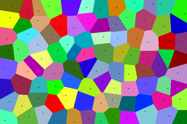
If an array of data was supplied to the input of the algorithm X , we will assume that each neuron is a “prototype” of data, which in some way personifies them. Neurons create a Voronoi diagram in the data space and predict the average value of the data instances in each cell.
The picture shows an example of a simple Voronoi diagram: the plane is divided into sections corresponding to points inside. The set inside each colored polygon is closer to the central point of this polygon than to other black points.
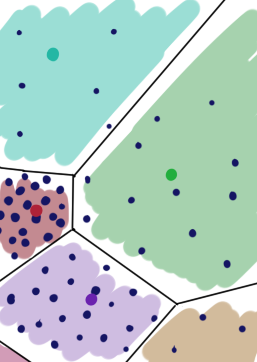
There is an important difference in the coverage of the GNG distribution of neurons: each section of the plane above has the same “price”. This is not the case for neural gas: zones with a high probability of occurrence x have more weight:
(The red neuron covers a smaller area because there are more data instances on it)
The errors accumulated at the stage (3) errori show how good neurons are in this. If a neuron frequently and heavily updates the weight, then either it doesn’t fit the data well, or it covers too much of the distribution. In this case, it is worth adding one more neuron so that it takes a part of the updates on itself and reduces the global discrepancy to the data. This can be done in different ways (why not just poke it next to the neuron with the maximum error?), But if we still consider the errors of each neuron, then why not apply some heuristics? See (9.1), (9.2) and (9.3).
Since the data is sent to the loop randomly, the error is a statistical measure, but as long as there are far fewer neurons than the data (and usually it is), it is quite reliable.
In the figure below, the first neuron approximates data well, its error will increase slowly. The second neuron badly approximates data because it is far away from them; it will move and accumulate an error. The third node badly approximates data, because it grabs off a distribution zone where there are several clusters, and not just one. It will not move (on average), but will accumulate an error, and sooner or later will generate a child node.
Pay attention to paragraph (9.5) of the algorithm. It should already be clear to you: the new neuron takes part of the data from its brethren under its wing u and v . As a rule, we do not want to insert new nodes several times in the same place, so that we reduce the error in u and v and give them time to move to a new center. Also do not forget about point (10). First, we do not want errors to increase indefinitely. Secondly, we prefer the new errors to the old ones: if the node, while traveling to the data, has accumulated a big mistake, after which it has fallen into the place where it is well approximating the data, then it makes sense to unload it a little so that it does not share in vain.
Weights and Ribs Update
Let's look at the scale weighting stage (4). Unlike gradient trigger algorithms (such as neural networks), which update everything at every step of the learning cycle, but little by little, neural gas and other SOM-like techniques concentrate on large-scale updating of weights only closest to vecx node and their direct neighbors. This is the strategy of Winner Takes All (WTA, the winner gets everything). This approach allows you to quickly find quite good w even with poor initialization, neurons receive large updates and quickly “reach” to the nearest data points. In addition, this way of updating gives the meaning of the accumulated errors. error .
If you remember how self-organizing cards work, you can easily understand where your ears grow from the idea of connecting nodes with edges (6). A priori information is transmitted to the SOM, as neurons should be located relative to each other. GNG does not have such initial data, they are searched on the fly. The goal, in part, is the same - to stabilize the algorithm, to make the distribution of neurons smoother, but more importantly, the constructed grid tells us exactly where to insert the next neuron and which neurons to delete. In addition, the resulting connection graph is invaluable at the stage of visualization.
Deleting nodes
Now a little more about the destruction of neurons. As mentioned above, by adding a node, we add a new “prototype” for the data. Obviously, some kind of restriction is needed on their number: although the increase in the number of prototypes is good from the point of view of data compliance, this is bad from the point of view of the benefits of clustering / visualization. What is the use of splitting, where there are exactly as many clusters as data points? Therefore, in GNG there are several ways to control their population. The first, the simplest - just a hard limit on the number of neurons (9). Sooner or later we stop adding nodes, and they can only shift to reduce the global error. Softer, the second - removal of neurons that are not associated with any other neurons (7) - (8). In this way, the old, outdated neurons, which correspond to the outliers, are removed, where the distribution has "disappeared" from, or that were generated in the first cycles of the algorithm, when the neurons still did not correspond well to the data. The more neurons, the more (on average) each neuron of the neighbors, and the more often the connections will grow old and decay, because at each stage of the cycle only one edge can be updated (they grow old, while all edges reach the neighbors).
Once again: if the neuron badly corresponds to the data, but still the closest one to them, it moves. If a neuron badly corresponds to the data and there are other neurons that best fit them, it never turns out to be a winner at the stage of updating the scales and sooner or later dies.
An important point: although this is not in the original algorithm, I highly recommend when working with rapidly and strongly varying distributions in step (5) to “age” all arcs, and not just arcs emanating from the winning neuron. The ribs between neurons that never win do not age. They can exist indefinitely, leaving ugly tails. Such neurons are easy to detect (it is enough to keep the date of the last victory), but they have a bad effect on the algorithm, depleting the pool of nodes. If you age all the edges, the dead nodes quickly ... well, they die. Minus: it tightens the soft limit on the number of neurons, especially when a lot of them accumulate. Small clusters may go unnoticed. Also need to put more amax .
Practical advice
As already noted, thanks to the WTA strategy, neurons receive large updates and quickly become good places even with bad starting positions. Therefore, there are usually no special problems with w1 and w2 - you can simply generate two random samples x and initialize neurons with these values. Also note that for the algorithm it is not critical that two and only two neurons are transmitted to it at the beginning: if you really want, you can initialize it with any structure you like, like SOM. But for the same reason, this makes little sense.
From the explanation above it should be clear that 0.5 leq alpha leq0.9 . Too small a value will not leave the parent neurons with absolutely no margin in the error vector, which means they will be able to generate another neuron soon. This can slow down GNG in the initial stages. With too large $ \ alpha $, on the contrary, too many nodes can be born in one place. This arrangement of neurons will require many additional iterations of the loop for adjustment. A good idea might be to keep u slightly more error than v .
In a GNG-devoted scientific article, it is advised to take the speed of learning the neurons of the winners in the range etawinner=0.01 dots0.3 . Alleged that etawinner=0.05 suitable for a variety of tasks as a standard value. The learning speed of the neighbors of the winner is advised to take one or two orders less than etawinner . For etawinner=0.05 can you stop at etaneighbor=0.0006 . The greater this value, the smoother the distribution of neurons will be, the less impact will be emitted, and the more willing neurons will be to drag on real clusters. On the other hand, too much etaneighbor may harm the already established correct structure.
Obviously, the larger the maximum number of neurons beta the better they can cover the data. As already mentioned, it should not be made too large, as this makes the end result of the algorithm less valuable to humans. If a R - the expected number of clusters in the data, then the lower bound on beta - 2 timesR (curious reader, think about how the statement “neurons survive in pairs” follows from the rule for removing neurons, and from it the assessment of beta ). However, as a rule, this is too small a quantity, because you need to take into account that not all the time neurons are good at bringing in data all the time - there must be a reserve of neurons for intermediate configurations. I could not find a study on optimal beta but good sighting number seems 8 sqrtdR or 12 sqrtdR if strongly elongated or nested clusters are expected.
Obviously, the more amax the more reluctant GNG will be to get rid of obsolete neurons. Too small amax the algorithm becomes unstable, too chaotic. When it is too big, it may take a lot of epochs to make neurons crawl from place to place. In the case of a time-varying distribution, neural gas in this case may not at all achieve even distant synchronism with the distribution. This parameter obviously should not be less than the maximum number of neighbors in a neuron, but its exact value is difficult to determine. Take amax= beta and deal with the end.
Difficult to give some advice on lambda . Both too large and too small a value are unlikely to damage the final result, but definitely more epochs will be required. Take lambda=|X|/4 , then move by trial and error.
About the number of epochs E it's pretty simple - the more the better.
I summarize that even though GNG has a lot of hyperparameters, even with a not very accurate set of them, the algorithm will most likely return you a decent result. It just takes him a lot more epochs.
Discussion
It is easy to see that, like SOM, Growing Neural Gas is not a clustering algorithm in itself; rather, it reduces the size of the input sample to a certain set of typical representatives. The resulting array of nodes can be used as a dataset map by itself, but it is better to run DBSCAN or Affinity Propagation, mentioned by me more than once, over it. The latter will be especially pleased with information about existing arcs between nodes.In contrast to self-organizing maps, GNG is well embedded in both hyper-balls and hyper-boxes, and can grow without additional modifications. What GNG is especially pleased with in comparison with its ancestor is that it does not degrade so much with increasing dataset dimensionality.
Alas, neural gas is not without flaws. First, purely technical problems: the programmer will have to work on the effective implementation of coherent lists of nodes, errors and arcs between neurons with insertion, deletion and search. Easy, but prone to bugs, be careful. Secondly, GNG (and other WTA algorithms) are paying off emissions sensitivity for large updates.W .In the next article and tell you how to smooth this problem a bit. Thirdly, although I mentioned the possibility of looking intently at the resulting graph of neurons, it is rather a pleasure for a specialist. In contrast to Kohonen maps, Growing Neural Gas alone is difficult to use for visualization. Fourth, GNG (and SOM) does not very well sense clusters of higher density within other clusters.
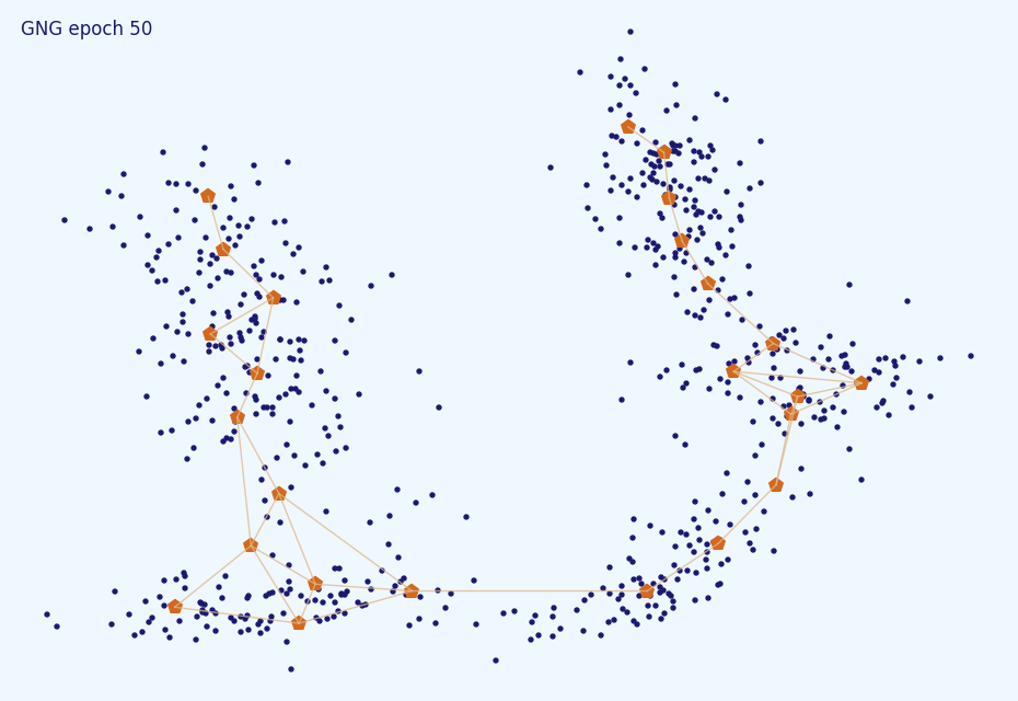
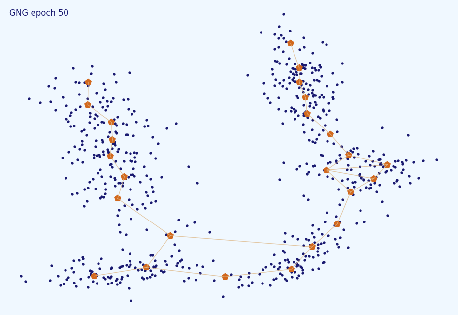
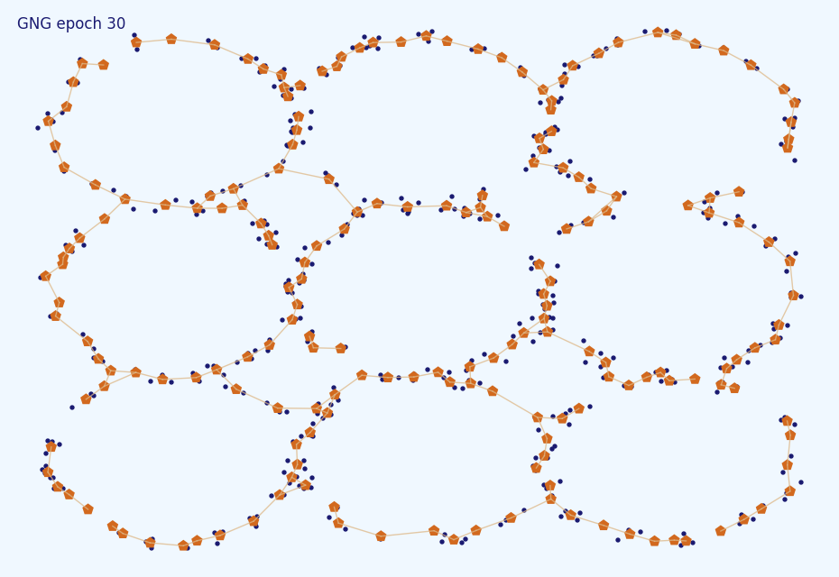
Under the spoiler pictures with examples of the algorithm
Pictures
, GNG :

, :
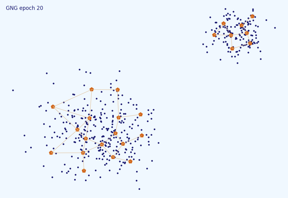

, . 10% :

:

GNG . learning rate (0.5), (1000) (5).

, . . ( amax=5 ):


Or maybe not. .
, . , , :

. , , , . , , :

, . — , , .
, :
, . 10% :
:
GNG . learning rate (0.5), (1000) (5).
, . . ( amax=5 ):
Or maybe not. .
, . , , :
. , , , . , , :
, . — , , .
Subtotal
In this article, we looked at the algorithm of the expanding neural view from a simplified and detailed point of view. We discussed the features of his work and the choice of hyperparameters. This should be enough for an independent implementation of the algorithm and effective work with it. Try to download my simple version from github and watch the animations in higher resolution at home or play around with the distributions here . Much of the article’s material was drawn from Jim Holmström's Growing Neural Gas wtih Utility. In the next article, I will highlight some of the weaknesses of the GNG and talk about modifications that are devoid of these shortcomings. Stay tuned!
Source: https://habr.com/ru/post/340360/
All Articles