Structure and randomness of prime numbers

Are primes scattered along the number axis like seeds scattered by the wind? Of course not: simplicity is not a matter of chance, but the result of elementary arithmetic. A number is simple if and only if no smaller positive integer except one divides it completely.

But the story does not end there. The distribution of primes looks random, with irregular discontinuities and clusters that look rather chaotic. If there is any scheme, then it is incomprehensible. In fact, primes look random enough to play dice with them. Create a list of consecutive primes (say, starting with 11, 13, 17, 19, ...) and divide them modulo 7. In other words, divide each prime number by 7 and save only the remainder. The result is a sequence of integers from the set {1, 2, 3, 4, 5, 6}, which looks almost like the result of several rolls of the correct bone.

$$

$$\ begin {align *} 11 \ bmod 7 & \ rightarrow 4 \ qquad 47 \ bmod 7 \ rightarrow 5 \\ 13 \ bmod 7 & \ rightarrow 6 \ qquad 53 \ bmod 7 \ rightarrow 4 \\ 17 \ bmod 7 & \ rightarrow 3 \ qquad 59 \ bmod 7 \ rightarrow 3 \\ 19 \ bmod 7 & \ rightarrow 5 \ qquad 61 \ bmod 7 \ rightarrow 5 \\ 23 \ bmod 7 & \ rightarrow 2 \ qquad 67 \ bmod 7 \ rightarrow 4 \\ 29 \ bmod 7 & \ rightarrow 1 \ qquad 71 \ bmod 7 \ rightarrow 1 \\ 31 \ bmod 7 & \ rightarrow 3 \ qquad 73 \ bmod 7 \ rightarrow 3 \ 37 \ bmod 7 & \ rightarrow 2 \ qquad 79 \ bmod 7 \ rightarrow 2 \\ 41 \ bmod 7 & \ rightarrow 6 \ qquad 83 \ bmod 7 \ rightarrow 6 \\ 43 \ bmod 7 & \ rightarrow 1 \ qquad 89 \ bmod 7 \ rightarrow 5 \\ \ end { align *}$$

Having worked with a larger sample (the first million prime numbers are greater than $$$10 ^ 7$ ), I calculated the number of primes with each of the six possible residues modulo 7 (also known as the six possible classes of congruence modulo 7). I also simulated a million throws in a hex bone. Can you say, looking at these two results, which of them is that?
')

                1 2 3 4 5 6
          166 787 166 569 166 714 166 573 166 665 166 692
              120 -98 47 -94 -2 25

                1 2 3 4 5 6
          166 768 166 290 166 412 166 638 167 282 166 610
              101 -377 -255 -29 615 -57

In each table, the first row indicates the number of results $$$x$ in each of the six classes. The second line shows the difference $$$x - \ bar {x}$ where $$$\ bar {x}$ - average value $$$1,000,000 / 6 = $ 166,66$ . In both cases, it seems that the numbers are distributed fairly evenly, with no obvious displacements. The first table shows the remains of prime numbers from division modulo 7. Their distribution is slightly flatter compared to the simulated bone and with smaller deviations from the mean; the standard deviation of the two samples is 84 and 346, respectively. Judging from these tables, it seems that any of the processes can be used to ensure the randomness required in a regular dice game.

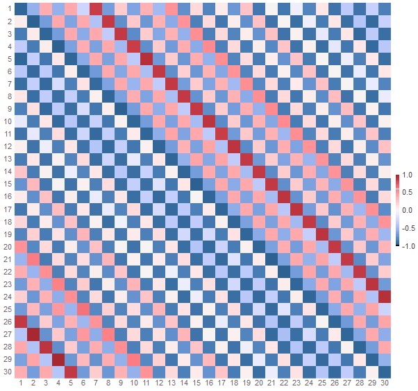
But the condition of randomness is not only a uniform distribution of results in the permissible interval. In addition, the individual events in the sequence must be independent of each other. One dice roll should not affect the result of the next roll. To test independence, you can look at successive events. How many times is there one more unit after unit, or deuce, or triple, and so on? Write in the matrix $$$6 × 6$ the number of all 36 possible pairs. If the process is indeed random, all 36 pairs must have the same frequency, if you do not take into account small statistical fluctuations. You can turn the matrix into a color “heat map”, in which cells with a number above the average will be displayed in warm shades of pink and red, and below the average - filled with cooler shades of blue. (Inserted quantities are not valid quantities. $$$x$ and the normalized variable $$$w = (x_ {i, \, j} - \ bar {x}, / \, \ bar {x}$ where $$$\ bar {x}$ - this is again the average value, in our case $$$1,000,000 / 36 = $ 27,77$ .) Here is a heat map of a simulated right bone:


Picture 1.

There is nothing interesting here. Almost all quantities are so close to the average that the cells of the matrix appear neutral gray, only a few turned pale pink or blue. It is this result that you expect when successive rolls of the dice do not correlate with each other, and all possible pairs are equally likely.

We now turn to the corresponding matrix of consecutive primes modulo 7:


Figure 2.

Wow! It looks like we left the Country of random numbers, here the old gray movie turned into Technicolor. A blue bar appeared on the heat map along the main diagonal (from the left top to the right bottom), meaning that successive pairs of prime numbers that have the same value of the remainder of dividing by 7 are very unlikely. In other words, couples $$$(1, 1), (2, 2), \ ldots (6, 6)$ occur less frequently than it would in a truly random sequence. The overdiagonal (directly above the main diagonal) has a lighter blue color. That means couples $$$(i, j)$ where $$$j = i + 1$ , occur a little less than the average frequency. For example, $$$(2, 3)$ and $$$(5, 6)$ have slightly negative normalized frequency values. On the other hand, the subdiagonal (under the main diagonal) is completely pink and red; couples like $$$(3, 2)$ or $$$(5, 4)$ where $$$j = i-1$ , occur with a frequency higher than average. Far from the diagonal, in the upper right and lower left corner we see a pastel chess pattern.

If you prefer to deal with numbers, rather than colored squares, then here is a matrix of values:

            pairs of consecutive prime numbers mod 7
                    1 2 3 4 5 6
           1 15656 24376 33891 29964 33984 28916
           2 37360 15506 22004 32645 25095 33959
           3 25307 41107 14823 22747 32721 30009
           4 32936 26183 37129 14681 21852 33791
           5 24984 34207 26231 41154 15560 24529
           6 30543 25190 32636 25382 37453 15488

Deviations from uniformity can be called whatever, but not “insignificant”. In the third row, for example, you can see that if you just met 3 in the sequence of mod 7 primes, then the next number is much more likely to be 2, and not another 3. If you were playing a game with bones from prime numbers, then such a shift would have a tremendous impact on the result. Bones on prime numbers - "charged" bones!

---

These remarkably strong correlations in pairs were discovered by Robert J. Lemke-Oliver and Kannan Sounararajan from Stanford University. They discussed them in a preprint published on arXiv in March of this year. For me, the most surprising thing about this discovery was that no one over the years has noticed these structures. They are pretty obvious if you know where to look.

I think it is impossible to blame Euclid for not finding them: in antiquity, ideas of chance and probability were not developed. But what about Gauss? He was a connoisseur of tables of prime numbers, and created his own lists of thousands of prime numbers. In his youth, he wrote : “one of my first projects was to observe a decreasing frequency of primes, for which I calculated several thousand primes ...” Moreover, Gauss practically invented the idea of ​​classes of congruence and modular arithmetic. But apparently, he never suspected that there might be something strange lurking in congruences of pairs of consecutive primes.

In the 1850s, Russian mathematician Pafnuti L. Chebyshev pointed out a slight distortion in prime numbers. Dividing odd primes modulo 4 divides them into two subsets. All prime numbers in the series 5, 13, 17, 29, 37, ... are congruent to 1 modulo 4; in the series 3, 7, 11, 19, 23, 31, ... congruent 3 modulo 4. Chebyshev noticed that prime numbers in the second category seem to be more numerous. For example, among the first 10,000 odd primes there are 4,943 congruent 1 and 5,057 congruent 3. However, this effect is small compared to the unevenness seen in pairs of consecutive primes.

In our time, several authors have seen a hint of the phenomenon of consecutive primes. Lemke Oliver and Soundararadzhan mention three such testimonies. (See the list of reference materials at the end of the article.) In the 1950s and 60s, Stanislav Knapowski and Pal Turan explored various aspects of the remnants of dividing prime numbers modulo m . In one article posthumously published in 1977, they considered the division of consecutive primes modulo 4 with residues 1 or 3. They "assumed" that consecutive pairs with the same residue and pairs with differing residues are "not equiprobable." In 2002, Chun-Min Ko investigated a series of consecutive primes (not just their pairs) and created elaborate fractal patterns based on their varying frequencies. Then, in 2011, Avner Ash and his colleagues published a detailed analysis of the “Frequencies of consecutive pairs of residuals of prime numbers,” including several matrices in which the diagonal decrease is clearly visible.

Given these precedents, were Lemke-Oliver and Soundararajan actually discovers the correlations of consecutive primes? In my opinion, the answer should be positive. Although others had seen these patterns before, they did not describe them so that they would be fixed in the minds of the mathematical community. In fact, when Lemke-Oliver and Sounondararajan announced their findings, the reaction was a surprise bordering on distrust. Erica Clararaich, in an article for Quanta, quoted the reaction of the Oxford number theorist James Maynard:

When Soundararajan first told Maynard about the opening of the pair, Maynard said, “I only half believed him. As soon as I returned to my office, I conducted a numerical experiment to verify this myself. ”

Obviously, this was a general reaction. In an article for Nature, Evelyn Lamb quotes Soundararajan: "Everyone we told about this, eventually wrote his computer program to see for himself."

I did the same! Over the past few weeks I have written a bunch of lines of code to analyze the division of prime numbers modulo m . My article is a report on my attempts to understand where these patterns come from. My methods are more computational and visual than mathematical, I can not prove anything. Lemke-Oliver and Soundararadzhan used a more rigorous and analytical approach, at the end of this article I will tell you a little more about their results.

If you want to start your own investigation, you can use my code as a basis. It is written in the Julia programming language , packaged in a Jupyter notebook, and is available on GitHub . (It so happened that this program was my first non-trivial experiment with Julia. In another article I will tell you more about my work with the language.)

---

In all the examples presented above, primes are divided by modulo 7, but in the number 7 there is nothing special. I chose it simply because the six possible residues {1, 2, 3, 4, 5, 6} correspond to the faces of an ordinary cubic bone. Other modules give similar results. Lemke-Oliver and Soundararajan most of the analysis was done on dividing the primes modulo 3, in which there are only two classes of congruences: a prime number greater than 3 should have a remainder of 1 or 2 when divided by 3. Here is a matrix of numbers for the first million prime numbers $$$10 ^ 7$ :

                              12
                     1 218578 281453
                     2 281454 218514 

Figure 3.

The pattern is pretty minimalistic, but still recognizable: elements outside the diagonal for sequences $$$(1, 2)$ and $$$(2, 1)$ more than the elements on the diagonal for $$$(1, 1)$ and $$$(2, 2)$ .

Prime numbers modulo 10 have four congruence classes: 1, 3, 7, 9. To see this, working in decimal notation, we do not even need arithmetic. When numbers are written at base 10, each prime number greater than 5 has a ending digit of 1, 3, 7, or 9. Here are the frequencies for 16 pairs of consecutive ending numbers:

                           1 3 7 9
                  1 43811 76342 78170 51644
                  3 58922 41148 71824 78049
                  7 64070 68542 40971 76444
                  9 83164 63911 59063 43924 

Figure 4.

The blue band is clearly visible along the main diagonal, although in other places of the matrix the pattern is slightly weakened and blurred.

I found that correlations between consecutive primes appear most clearly when the module itself is a prime number, and not too small. Look at the heat maps for successive prime numbers mod 13 and mod 17:


Figure 5.


Figure 6.

What about module 31?


Figure 7.

From these matrices you get a great pattern for a kilt or a mosaic floor, right? And in all of them there are interesting patterns. Diagonal stripes stand out not only on the main diagonal, but also in the entire matrix. Such stripes also create a checkerboard pattern. Along any row or column, cells are usually alternately red and blue. A more invisible feature is the approximate two-sided symmetry along the opposite diagonal (going from left bottom to right top). If you add a square along this line, then the cells joined together will be approximately the same color. (This fact was noticed by Ash and his co-authors.)

For further analysis, I decided to focus on successive mod 19 primes. The module is large enough to result in well-differentiated bands, but not so large as to make the matrix huge.


Figure 8.

How to understand the meaning of what we see? We begin the observation that all the primes in our sample are odd, and therefore all the intervals between these primes are even numbers. For any given simple $$$p$ the next candidates for the title of prime are $$$p + 2, p + 4, p + 6, \ ldots$ . Is this somehow connected with a chessboard pattern? If the steps between prime numbers must be multiples of 2, this can certainly create correlations between every second cell of any column or row. (Indeed, the correlations with the cell should be clearly visible through time - all even elements should be zero if the module would be an even number. Even cells can be filled only by “cyclic return” of the edge of the matrix to the odd border.)

Diagonal bands in the matrix suggest a strong correlation between all pairs separated by a certain numerical interval. For example, the dark blue diagonal and the brightest red diagonal consist of cells separated by six elements along the j axis. The first line contains cells 1 and 7, then 2 and 8, 3 and 9, and so on. It seemed to me that this relationship is easier to perceive if the matrix is ​​“bent” so that the diagonals become columns. The idea is to apply a cyclic shift to each line, all values ​​in the line will shift to the left, and those that “fall” from the left edge will be inserted to the right. The first line is shifted to zero positions, the next - one position, and so on. (Is there a name for this transformation? I’ll just call it “bend.”)

Then I wrote the code for this transformation, but as a result I didn’t get exactly what I expected:


Figure 9.

What are these zigzags along the reverse diagonal? I assumed that I made a mistake and shifted an extra element by one. And the root of the problem really turned out to be this, but the “bug” is not in the algorithm, but in the data itself. The matrices shown by me in all the previous drawings are only partial, they discard empty classes of congruence. In particular, the matrix for pairs of primes modulo 19 ignores all primes congruent to 0 modulo 19 on the logical basis that there are no such primes. In the end, if $$$p> 19$ and $$$p \ equiv 0 \ bmod 19$ then $$$p$ cannot be simple, because it is divisible by 19. However, the row and column for $$$p \ equiv 0 \ bmod 19$ are the real part of the matrix. If we add them, our color-coded scoreboard will look like this:


Figure 10.

The presence of a null row and column makes the definition of bending more accurate: for each row $$$i$ apply cyclic left shift to $$$i$ places The resulting curved matrix also looks neater:


Figure 11.

What do these vertical stripes tell us? In the original matrix element $$$i, j$ represented the frequency with which $$$i \ bmod 19$ follows $$$j \ bmod 19$ . Here is the cell color $$$i, j$ denotes the frequency with which $$$i \ bmod 19$ follows $$$(i + j) \ bmod 19$ . In other words, each column combines elements with the same mod 19 interval between two prime numbers. For example, the leftmost column contains all pairs separated by an interval of length $$$0 \ bmod 19$ and the bright red column in $$$j = 6$ considers all cases where consecutive primes are separated from each other $$$6 \ bmod 19$ .

Color coding gives us a good idea of ​​which intervals appear more or less often. For a more accurate quantitative measurement, we can summarize along the columns and display the results in a bar graph:


Figure 12.

Three observations:

• The uneven even-odd numbers observed above are clearly visible on the graph. With the exception of 0, each even interval is allocated against its odd neighbors.
• The interval between prime numbers mod 19, equal to 6 - the most popular of all. Numbers that are multiples of 6 (namely, 12 and 18) are also frequent, but at least to a lesser degree.
• The interval between prime numbers mod 19, equal to 0, is remarkably not popular. These are elements along the main diagonal of the original matrix, so it is not surprising that their sum is at the bottom, but the deficit is stronger than I expected.

I wanted to understand the sources of these patterns. What makes interval 6 so appealing to pairs of consecutive primes, and why almost all primes eschew the poor interval 0?

I already have a remote guess regarding popularity 6. In the 1990s, Andrew Odlyzhko, Michael Rubinstein and Marek Wolfe performed a computational study of “jumping champions” among prime numbers:

An integer D is called a jump champion if its most frequently occurring difference between consecutive primes ≤ x for some x .

Among the smallest prime numbers ( x is less than about 600), the jump champion is usually 2, but then wins 6 and dominates over a rather large interval of the number axis. About$$x = 10 35 number 6 inferior championship 30, which eventually gives 210. Odlyzhko and colleagues estimated that this last transition occurs approximately$x = 10^{35}$$$$x = 10^{425}$ .The numbers in this jump champion sequence - 2, 6, 30, 210, ... - are primeals ; The n th prime is the product of the first n prime numbers.

Why do primoryals become the preferred intervals between consecutive prime numbers? If a $$p is a sufficiently large prime number, then$p$$$p + 2 cannot be divisible by 2,$p + 2$$$p + 6 cannot be divisible by 2 and 3,$p + 6$$$p + 30 cannot be divisible by 2, 3, and 5, and in general$p + 30$$$$p + P_{n}$ where $$P n is then-th prime, not divisible by any of the firstnprime numbers.$P_{n}$ Of course $$p + P n can still be divided into some large prime number, or there may be another prime number between$p + P_{n}$$$$p$ and $$p + P n , such that the interval between primes is not guaranteed to be prime. But these intervals have an advantage over other applicants. We can see this rationale in action by taking the difference between the consecutive elements of our list of a million eight-bit prime numbers and plotting their frequencies:$p + P_{n}$




Figure 13.

Again, the interval of 6 stands out clearly, amounting to 13.7% of the total, the larger multiples of 6 also stand out among their immediate neighbors. It is worth noting the general shape of the distribution: a cluster on the left (with a peak on the number 6), followed by a gradual decrease. The trend is similar to the Poisson distribution, and in fact it can be considered a valid description.

Color scheme cuts a lot of data on the proportion of19 values ​​each. The blue fraction, which includes the intervals between primes ranging in length from 0 to 18, accounts for 68 percent of all the intervals present in a sample of one million prime numbers; the gold share adds another 23 percent. The remaining 9 percent is distributed widely and evenly. Not all intervals are shown on the graph: the spectrum extends to 210. (One pair of consecutive primes in the sample has a distance of 210, namely 20 831 323 and 20 831 533.)

It looks like Figure 13 shows the majority of the pattern of consecutive prime numbers modulo 19. I can make the schedule even more informative by making a simple change. We will begin to shift each beat of the 19 elements until it aligns with the beat of 0, gathering in bars that are in one column. Since the second (golden) share moves to the left until column 19 aligns with column 0, and the third (pink) share connects column 38 with column 0. Physically, this process can be thought of as rotating the graph around a cylinder with a circumference of 19. Mathematically it makes a division the intervals between primes modulo 19.


Figure 14.

If you do not pay attention to too bright colors, Figure 14 is similar to Figure 12: the heights of all columns are the same. This should not surprise us. In Figure 12, we divide prime numbers modulo 19, and then take the differences between consecutive divided primes. In Figure 14, we take the differences between the primes themselves, and then divide these differences modulo 19. The two procedures are similar:

$$

$$(p \bmod 19 - q \bmod 19) \bmod 19 = (p - q) \bmod 19.$$

Having studied the colors, we can place all the pieces of the puzzle in place. Why are primes mod 19 so often separated by an interval of 6? Well, actually mod 19 has little to do with this; the number 6 itself in this sample is the most frequent interval between prime numbers. The only other significant contribution to$$$\delta \equiv 6 \bmod 19$arises from the third beat, especially several pairs of prime numbers with a distance of 44. The

superiority of the first beat also explains the inequality between even and odd intervals. All intervals in the first beat necessarily even, odd intervals (mod 19) begin to appear only in the second beat (intervals from 19 to 37) and for this reason alone they are less frequent. For eight-digit prime numbers, the samples are more than two-thirds of consecutive pairs closer than 19 units, and therefore are in the first beat. (The median distance between prime numbers is 12. The average interval is equal to 16.68, which is close to the theoretical prediction of 16.72.)

Finally, Figure 14 can tell us something about the rarity of the 0 mod 19 intervals. No two consecutive prime numbers can fall into one class of the mod 19 congruence, unless they are separated by a distance of 38 or a multiple of 38. Therefore, such pairs are not they go on stage before the beginning of the third beat, and there cannot be too many of them in it. A sample of one million prime numbers contains 8,384 consecutive pairs with a distance of 38 — less than one percent of the total. And this is the main reason that the bone of primes so rarely falls the same face twice in a row. This is the reason for the appearance of the blue diagonal strip in all matrices.

---

I find it very interesting that we can explain so much about the pattern of successive mod m prime numbers without going into details and not considering the special properties of prime numbers. In fact, we can recreate a significant part of the pattern without using prime numbers at all.

Two hundred years ago, Gauss and Legendre noticed that, next to the number$$$x$ the fraction of all integers that are simple is approximately $$$1 / \log x$ .In 1936, the Swedish mathematician Harald Kramer suggested interpreting this fraction as a probability. The idea was to go through all the integers in order, taking each$$$x$ with probability $$$1 / \log x$ .The numbers in the accepted set will not be prime, except by coincidence, but they will have the same large-scale distribution as the prime number distribution. Here are the first few items in the million list of such “Cramer primes”, where the process of random selection begins with$$$x = 10^7$ :

 10000007
     10000022
     10000042
     10000065
     10000068
     10000098
     10000110
     10,000,116
     10000119
     10,000,128
     10,000,166 

Now suppose that we skip these numbers through the same mechanism that was applied to primes. We divide each Kramer prime number modulo 19, and then create a matrix of subsequent numbers$$$19 × 19$ :


Figure 15.

The prominent diagonal features look similar, but they are much simpler than in the corresponding prime number graphs. For any Kramer prime number p mod 19, the most likely follower is p + 1 mod 19, and the least likely one is p + 19 mod 19. Between these limiting cases there is a smooth frequency or probability gradient with only a few small fluctuations, which you can most likely write off for statistical noise.

This matrix is ​​missing only a chess pattern. We can partially restore its structure by generating a new set of numbers, which I call the “Cramer semi-simple numbers”. They are created by the same probabilistic sifting of integers, but this time we consider only odd numbers as candidates and change the probability to$$$2\, / \log x$ To keep the same density:


Figure 16.

That's better! With the exclusion of even numbers from the sequence, the minimum interval between semisimple numbers is 2, and this is also the most likely location.

By adding another change, we will get even closer to imitating the matrix of true primes. In addition to eliminating all integers that are multiples of 2, we also get rid of multiples of 3 and change the probability of the sample accordingly. We call the resulting numbers "semi-simple Cramer numbers."


Figure 17.

Notice that 6 mod 19 is the most likely interval between Cramer's semi-semi-simple numbers, as well as between true primes, and that the same echoes are present at intervals of 12 and 18. Indeed, the only obvious difference between this matrix and Figure 10 (the corresponding graph for true prime numbers) is in the column and row for numbers congruent to 0 modulo 19. There cannot be such numbers among prime numbers. If we eliminate them from the Kramer numbers, then the two matrices become almost indistinguishable. Here they are both:


Figure 18.

If you look closely, you can find differences - look at the expansion of the diagonal to the south-east of row 1, column 15 - but in general, these modified Cramer numbers mimic surprisingly well simple numbers. In both diagrams, even symmetry with respect to the inverse diagonal is noticeable. And do not forget that these two sets contain in total only 19 percent of their values: Cramer numbers include 189,794 true primes.

---

I want to add another twist to the story. All the examples above are based on prime numbers (or their analogs) of eight decimal digits, or, in other words, numbers next to$$$10^7$ . Are the same results for primes with higher values? Consider a table created from successive pairs of a million 40-bit prime numbers taken modulo 19. The pattern is familiar, but more pale:


Figure 19.

Let us turn to prime numbers from 400 digits, again divided modulo 19, and we obtain colors that have faded almost beyond recognition:


Figure 20.

The blue stripe on the main diagonal is hardly distinguishable, and the other features turn into simple random spots.

So it seems that for pairs of consecutive primes, size matters. To understand the reasons for this, let's look at a group of differences between consecutive prime numbers in a 40-bit sample:


Figure 21.

Compared with the distribution of intervals for eight-bit prime numbers (Figure 13), the spectrum is much wider and flatter. In this form, the graph is truncated in the interval 240; the long “tail” actually stretches far to the right, and the largest gap between consecutive primes is 1,328. Also, as Odlyzhko predicted with his colleagues, the most frequent interval between 40-bit prime numbers is not 6, but 30.

Due to the wider distribution of intervals, the first beat cannot dominate the behavior of the system as it does among eight-digit prime numbers. When we start placing one modal portion over another, mod 19 (Figure 22 below), the first six or eight segments make a significant contribution. The unevenness of even-odd is still present, but the amplitude of these oscillations is much reduced. The leftmost column of the graph, representing the intervals congruent to 0 modulo 19, is stunted in growth, but not so significantly.


Figure 22.

Spectrum alignment becomes even more pronounced in a sample of one million 400-bit prime numbers:


Figure 23.

Now the gaps between prime numbers stretched to 15,080, creating almost 800 shares of mod 19 (however only 13 are shown). And here in the array there is a very intriguing comb structure. In general, columns on numbers that are multiples of 6 stand out almost twice compared to the height of the nearest neighbors, showing the persisting influence of the smallest prime factors 2 and 3. The numbers that are multiples of 6, which are also multiples of 30, reach even greater heights. The values ​​in the sequence 42, 84, 126, 168, 210, ... also contribute greatly: these numbers are multiples of $$$42 = 2 × 3 × 7$ . And note that 210, which is a multiple of 6 and 30 and 42, is a new champion interval, again confirming Odlyzhko’s forecast.

Despite all this internal structure, when the columns are placed one upon another in mod 19, the mixture 800 is so neat that the heights are almost the same. The only thing that remains is a small unevenness of even-odd.


Figure 24.

And the chronically unpopular class of congruent 0 modulo 19 intervals finally found an equal. Most of the column height is not from a dozen early longs, but from hundreds of later ones, representing intervals between 228 and 15 080 (they all accumulated in the turquoise region of the graph).

---

Experiments with large prime numbers allow us to make a plausible assumption: as the size of prime numbers tends to infinity, all traces of correlations gradually fade, and successive pairs of prime numbers will be as random as throws of an ideal dice. But is it? There are several reasons to be skeptical of this hypothesis. First, if we increase the modulus m together with the size of the primes, making it comparable in magnitude with the median gap between primes, then the correlations will still appear. In my 40-bit sample, the median gap between primes is 66, so let's consider the matrix of mod 61 consecutive pairs. (To limit statistical noise, I will perform calculations with a sample of ten million 40-bit prime numbers).


Figure 25.

The bands are back! And in fact, in addition to the familiar bright red stripes at intervals of 6, there are more diffuse pink and blue frequencies with a period of 30. I would like to look at the matrix for simple 400-bit numbers, which may have even more complex features, with interacting waves in periods 6, 30 and 210. Unfortunately, I can not show you this drawing. The median gap between 400-bit prime numbers is approximately 640, so we have to assign m a value equal to a prime number in this interval, say 641. To fill the matrix $$$641 × 641$ It takes about a billion consecutive 400-bit numbers, which is more than I’m ready to calculate.

There are other reasons to doubt that with increasing primes, the correlations completely disappear. The comb structure, so noticeable in Figures 21 and 23, tells us that the rule of divisibility into small primes strongly influences the distribution of large primes mod m , and this influence still does not disappear when the numbers increase. Moreover, even when m is much smaller than the median interval between prime numbers, the blue bar remains weakly visible. Here is the matrix for pairs of consecutive 400-bit mod 3 primes:

                              12
                     1 248291 251128
                     2 251127 249453 

The difference of elements on the diagonals and outside the diagonals is much smaller than with eight-digit prime numbers (compare with Figure 3), but the deviations still do not look like random variation.

To get a clearer idea of ​​how the correlation changes as a function of the size of primes, I decided to create a sample of primes over the entire range from single-digit to 400-bit numbers. In this project, I decided to do better than Gauss: he put simple numbers in the chiliad tables (in groups of 1,000), and I calculated them in myriads (groups of 10,000). To measure the correlations among the prime numbers mod m, I calculated the average value of the diagonal elements of the matrix and the average of the elements outside the diagonals, and then took the ratio out / on the diagonal. If consecutive primes are completely uncorrelated, the ratio should tend to 1.

Figure 26 shows the result for 797 myriad mod 3 prime numbers. The curve is curved upward, has a sharp initial decline, and then a much flatter segment. Starting at around 100 bits, there are samples with a ratio of less than 1, meaning that the diagonal is more densely populated than areas outside the diagonal. But even at 400 bits, most of the ratios are still above 1. What do we see here? Is the curve approaching a ratio of 1 slowly, or is there a limiting value slightly larger than 1? Unfortunately, computational experiments do not give a definitive answer.


Figure 26.

---

For consideration of this problem in the article by Lemke-Oliver and Soonararajan, other tools are used. Although they use numerical studies, their goal is to find an analytical solution. A goal is a mathematical function or formula whose input data are four positive integers: m is the module, a and b are the congruence classes of primes mod m , and x is the upper limit of the size of primes. The formula should show us how often a followed by b among all primes less than x follows a. If we had such a formula, we could color all the squares in the matrix of consecutive numbers $$$m × m$ without the need to even calculate the prime numbers themselves up to x .

Describing the behavior of all primes up to x is a much more difficult task than taking a sample of primes next to x . The analytical approach is complicated for other reasons: it requires ideas, and not just CPU cycles. But the reward can potentially be much more valuable. For example, calculating the equation $$$A = \ pi r ^ 2$ , we get the true values ​​for all circles, something that a finite number of calculations cannot give us (with a finite approximation to $$$\ pi$ ). This promises us not only to obtain strict solutions, but the emergence of insights.

Alas, I did not manage to get insight from the reading analysis of Lemke-Oliver and Sounondararajan. Basically, the gaping gaps in my knowledge of analytic number theory are to blame, but I think it will be fair to say that in some parts of the article mathematics becomes rather frightening. The equation below is the main hypothesis of Lemke-Oliver and Soundararajan. (I slightly changed its notation and simplified one aspect of the equation: the original is applicable to a series of r consecutive prime numbers, but in my version only pairs are described, i.e. $$$r = 2$ .)

$$

$$\ pi (x; m, a, b) = \ frac {\ mathrm {li} (x)} {\ phi (m) ^ 2} \ left (1 + c_1 (m; a, b) \ frac { \ log \ log x} {\ log x} + c_2 (m; a, b) \ frac {1} {\ log x} + O \ Big (\ frac {1} {(\ log x) ^ {7 / 4}} \ Big) \ right)$$

I think I understand well enough what is happening here to offer my explanations. To the left of the equal sign $$$\ pi (x; m, a, b)$ denotes a counting function, while $$$\ pi (x)$ counts primes to $$$x$ , $$$\ pi (x; m, a, b)$ Is the number of pairs of consecutive primes $$$m$ falling into congruence classes $$$a$ and $$$b$ . To the right of the equal sign the main factor $$$\ mathrm {li} (x) / \ phi (m) ^ 2$ is the average or expected number of pairs if the primes were randomly evenly distributed without correlations between consecutive primes; $$$\ mathrm {li} (x)$ Is a logarithmic integral $$$x$ approximation $$$\ pi (x)$ , but $$$\ phi (m) ^ 2$ Is the Euler function, which considers the square of the number of possible classes of congruences for \ (m \), or, in other words, the number of elements in the matrix of consecutive numbers.

The main term in large brackets is just $$$1$ and therefore it appends the value of the main coefficient $$$\ mathrm {li} (x) / \ phi (m) ^ 2$ ; so the average number of pairs $$$(a, b)$ becomes the first approximation to the counting function. The following three terms are used to refine this first approximation; for big $$$x$ they should get smaller because $$$\ log \ log x / \ log x \ gt 1 / \ log x \ gt 1 / (\ log x) ^ {7/4}$ at $$$x \ gt e ^ e \ approx 15$ .

What about the coefficients of these three clarifying members? Record $$$O \ cdot$ for the smallest member means that we will be interested only in the order of magnitude of the member, which for a large $$$x$ will be small. Coefficient $$$c_1$ at $$$r = 2$ takes the following form:

$$

$$c_1 (m; a, b) = \ frac {1} {2} - \ frac {\ phi (m)} {2} (\ # \ {a \ equiv b \ bmod m \})$$

Expression $$$\ # \ {a \ equiv b \ bmod m \}$ counts the number of times when $$$a$ and $$$b$ belong to one class of congruence mod $$$m$ . That is, the importance of a member (if I understood correctly) is to reduce the total number along the diagonal of the matrix, where $$$a \ equiv b \ bmod m$ .

As for the ratio $$$c_2$ , Lemke-Oliver and Soonararajan point out that “in general, [it] seems difficult.” And they are right. At this point, I should advise readers who want to learn more, read the original article on their own.

The complexity of the mathematical description frustrates me, but very often a simply formulated task requires a deep and complex solution. I have only hope that after additional work some of the technical details can be discarded, and the basic ideas will be clearer. In the meantime, we can still explore the fascinating and long-hidden corner of the theory of numbers with the help of simple computing tools, as well as drops of graphics.

“God may not play dice with the Universe, but something strange happens with prime numbers,” said Pal Erdös and / or Mark Katz, with a little help from Karl Pomerans . The strangeness is manifested strangest of all when we play dice with the help of prime numbers.

Addition. I mentioned above that the distribution of prime numbers modulo 7 seems flatter or more close to uniform than the result of throwing a regular dice. John D. Cook conducted a chi-square check with the data and it turned out that they fit into a uniform distribution too well to be a plausible result of a random process. In his first post , a specific case of prime numbers modulo 7 is considered; in his second post other modules are considered.

---

Reference materials

Ash, Avner, Laura Beltis, Robert Gross, and Warren Sinnott. 2011. Frequencies of success pairs of prime residues. Experimental Mathematics 20 (4): 400–411.
Chebyshev, Pafnuty Lvovich. 1853. Lettre de M. le Professeur Tchébychev à M. Fuss sur un nouveaux théorème relatif aux nombres premiers contenus dans les formes 4 n + 1 et 4 n + 3. Bulletin de la Academie de l'Academie Imperiale des Sciences de Saint-Pétersbourg 11: 208. Google books

Cramér, Harald. 1936. On the order of magnitude between consecutive prime numbers. Acta Arithmetica 2: 23–46. PDF

Derbyshire, John. 2002. Chebyshev's bias .

Granville, Andrew. 1995. Harald Cramér and the distribution of prime numbers. Harald Cramér Symposium, Stockholm, 1993. Scandinavian Actuarial Journal 1: 12–28. PDF

Granville, Andrew, and Greg Martin. 2004. Prime number races. arXiv

Hamza, Kais, and Fima Klebaner. 2012. On the statistical independence of primes. The Mathematical Scientist 37: 97–105.

Klarreich, Erica. 2016. Mathematicians discover prime conspiracy. Quanta .

Knapowski, S., and P. Turán. 1977. On prime numbers? 1 resp. 3 mod 4. In Number Theory and Algebra: Collected Papers Dedicated to Henry B. Mann, Arnold E. Ross, and Olga Taussky-Todd , pp. 157–165. Edited by Hans Zassenhaus. New York: Academic Press.

Ko, Chung-Ming. 2002. Distribution of the numbers of primes. Chaos Solitons Fractals 13 (6): 1295–1302.

Lamb, Evelyn. 2016. Peculiar pattern found in 'random' prime numbers. Nature doi: 10.1038 / nature.2016.19550.

Lemke Oliver, Robert J., and Kannan Soundararajan. 2016 preprint. Unexpected biases in the distribution of consecutive primes. arXiv

Odlyzko, Andrew, Michael Rubinstein, and Marek Wolf. 1999. Jumping champions. Experimental Mathematics 8 (2): 107–118.

Rubinstein, Michael, and Peter Sarnak. 1994. Chebyshev's bias. Experimental Mathematics 3: 173–197. Project euclid

Tao, Terrence. Structure and randomness in the prime numbers. PDF