Deep learning with R and Keras on the example of the Carvana Image Masking Challenge

Much more attractive is the use of R-interfaces to TensorFlow and Keras with backends to choose from (TensorFlow, Theano, CNTK), detailed documentation and many examples. In this message, the solution of the problem of image segmentation will be analyzed on the example of the Carvana Image Masking Challenge competition ( winners ), in which you want to learn how to separate cars photographed from 16 different angles from the background. The "neural network" part is fully implemented on Keras , magick is responsible for image processing (interface to ImageMagick ), parallel processing is provided by parallel + doParallel + foreach (Windows) or parallel + doMC + foreach (Linux).

Content:

1. Installation of all necessary
2. Imaging: magick as an alternative to OpenCV
3. Parallel code execution on R in Windows and Linux
4. reticulate and iterators
5. The segmentation task and loss function for it
6. U-Net architecture
7. Model training
8. Model based predictions

1. Install all the necessary

We assume that the reader already has a Nvidia GPU with ≥4 GB of memory (less possible, but not so interesting), and the CUDA and cuDNN libraries are installed. For Linux, the installation of the latter is simple ( one of numerous manuals ), and for Windows it is even easier (see the section "CUDA & cuDNN" in the manual ).

Next, it is desirable to install the Anaconda distribution with Python 3; To save space, you can choose the minimum option Miniconda. If suddenly the Python version in the distribution kit is ahead of the latest version supported by Tensorflow, you can replace it with a command like conda install python=3.6 . Also, everything will work with regular Python and virtual environments.

The list of used R-packages is as follows:

 library(keras) library(magick) library(abind) library(reticulate) library(parallel) library(doParallel) library(foreach) 

 library(keras) library(magick) library(abind) library(reticulate) library(parallel) library(doMC) library(foreach) 

All of them are installed with CRAN, but Keras is better to take from Github: devtools::install_github("rstudio/keras") . The subsequent launch of the install_keras() command will create a conda environment and install the correct versions of Python's Tensorflow and Keras in it . If for some reason this command refused to work correctly (for example, it could not find the desired Python distribution), or specific versions of the used libraries are required, you should create a conda-environment yourself, install the necessary packages in it, and then in R specify the package to reticulate This is the environment with the use_condaenv() command.

The list of parameters used further:

 input_size <- 128 #    ,     epochs <- 30 #   batch_size <- 16 #   orig_width <- 1918 #    orig_height <- 1280 #    train_samples <- 5088 #    train_index <- sample(1:train_samples, round(train_samples * 0.8)) # 80% val_index <- c(1:train_samples)[-train_index] #    images_dir <- "input/train/" masks_dir <- "input/train_masks/" 

2. Working with images: magick as an alternative to OpenCV

When solving machine learning tasks on graphic data, one should be able to, at a minimum, read images from a disk and transfer them to the neural network in the form of arrays. Usually it is also required to be able to perform various image transformations in order to implement the so-called augmentation - the addition of a training sample with artificial examples created from the samples actually present in the training sample itself. Augmentation is (almost) always capable of increasing the quality of a model: basic understanding can be obtained, for example, from this message . Looking ahead, we note that all this needs to be done quickly and multi-threaded: even on a relatively fast CPU and a relatively slow video card, the preparatory stage may be more resource-intensive than the actual training of the neural network.

In Python, OpenCV is traditionally used to work with images. Versions of this megablibrary for R have not yet been created, calling its functions through reticulate looks like an unsportsmanlike decision, so we will choose from the available alternatives.
The top 3 most powerful graphics packages are as follows:

• EBImage - a package created using S4-classes and placed in the Bioconductora repository, which implies the highest quality requirements for both the package itself and its documentation. Unfortunately, to enjoy the extensive capabilities of this software product is hampered by its extremely low speed of work.

  
  

• imager - this package looks more interesting in terms of performance, since the main work in it is performed by compiled code in the person of the CImg sishnoy library. Among the advantages can be noted the support of the "conveyor" operator %>% (and other operators from magrittr ), tight integration with packages from the so-called. tidyverse , including ggplot2 , as well as support for the split-apply-combine ideology. And only an incomprehensible bug that makes the functions for reading pictures on some PCs inoperable prevented the author of this message from choosing this package.

  
  
• magick is a wrapper for ImageMagick , developed and actively developed by members of the rOpenSci community. Combines all the advantages of the previous package, stability, glitch-free and killer feature (useless as part of our task) in the form of integration with the Tesseract OCR library. Measurements of speed when performing reading and transformation of pictures on a different number of cores are given below. Of the minuses, the esoteric syntax can be noted in places: for example, for trimming or resizing, you need to pass a "100x150+50" string to the function instead of the usual arguments like height and width . And since our auxiliary functions for preprocessing will be parameterized just by these values, we will have to use ugly paste0(...) or sprintf(...) constructions.

Hereinafter, we will generally reproduce the Kaggle Carvana Image Masking Challenge solution with Keras from Peter and Giannakopoulos.

You need to read the files in pairs - the image and the corresponding mask; you should also apply the same transformations to the image and the mask (turns, shifts, reflections, zoom) when using augmentation. We implement reading in the form of a single function, which will immediately reduce the image to the desired size:

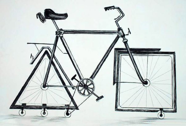
 imagesRead <- function(image_file, mask_file, target_width = 128, target_height = 128) { img <- image_read(image_file) img <- image_scale(img, paste0(target_width, "x", target_height, "!")) mask <- image_read(mask_file) mask <- image_scale(mask, paste0(target_width, "x", target_height, "!")) list(img = img, mask = mask) } 

The result of the function with the imposition of a mask on the image:

 img <- "input/train/0cdf5b5d0ce1_01.jpg" mask <- "input/train_masks/0cdf5b5d0ce1_01_mask.png" x_y_imgs <- imagesRead(img, mask, target_width = 400, target_height = 400) image_composite(x_y_imgs$img, x_y_imgs$mask, operator = "blend", compose_args = "60") %>% image_write(path = "pics/pic1.jpg", format = "jpg")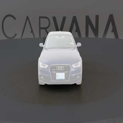 

The first type of augmentation will be a change in brightness (brightness), saturation and hue. For obvious reasons, it applies to a color image, but not to a black and white mask:

 randomBSH <- function(img, u = 0, brightness_shift_lim = c(90, 110), # percentage saturation_shift_lim = c(95, 105), # of current value hue_shift_lim = c(80, 120)) { if (rnorm(1) < u) return(img) brightness_shift <- runif(1, brightness_shift_lim[1], brightness_shift_lim[2]) saturation_shift <- runif(1, saturation_shift_lim[1], saturation_shift_lim[2]) hue_shift <- runif(1, hue_shift_lim[1], hue_shift_lim[2]) img <- image_modulate(img, brightness = brightness_shift, saturation = saturation_shift, hue = hue_shift) img } 

This conversion is applied with a 50% probability (in half of the cases the original image will be returned: if (rnorm(1) < u) return(img) ), the amount of change for each of the three parameters is randomly selected within the range of values ​​specified as a percentage of the original magnitude.

Also, with a probability of 50%, we will use horizontal reflections of the image and masks:

 randomHorizontalFlip <- function(img, mask, u = 0) { if (rnorm(1) < u) return(list(img = img, mask = mask)) list(img = image_flop(img), mask = image_flop(mask)) } 

Result:

 img <- "input/train/0cdf5b5d0ce1_01.jpg" mask <- "input/train_masks/0cdf5b5d0ce1_01_mask.png" x_y_imgs <- imagesRead(img, mask, target_width = 400, target_height = 400) x_y_imgs$img <- randomBSH(x_y_imgs$img) x_y_imgs <- randomHorizontalFlip(x_y_imgs$img, x_y_imgs$mask) image_composite(x_y_imgs$img, x_y_imgs$mask, operator = "blend", compose_args = "60") %>% image_write(path = "pics/pic2.jpg", format = "jpg")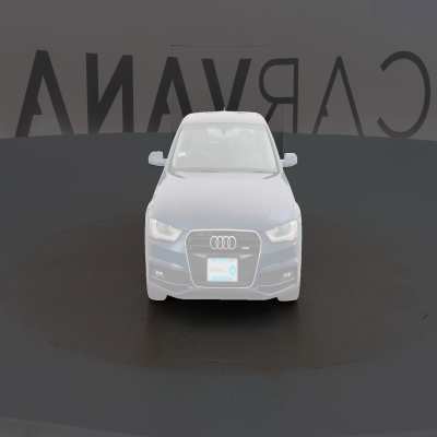 

The remaining transformations for the further presentation are not fundamental, therefore we will not dwell on them.

The last stage is the transformation of images into arrays:

 img2arr <- function(image, target_width = 128, target_height = 128) { result <- aperm(as.numeric(image[[1]])[, , 1:3], c(2, 1, 3)) # transpose dim(result) <- c(1, target_width, target_height, 3) return(result) } mask2arr <- function(mask, target_width = 128, target_height = 128) { result <- t(as.numeric(mask[[1]])[, , 1]) # transpose dim(result) <- c(1, target_width, target_height, 1) return(result) } 

Transposing is necessary so that the image lines remain rows in the matrix: the image is formed line by line (as the scanning beam moves in the kinescope), while the matrices in R are filled in columns (column-major, or Fortran-style; for comparison, in numpy you can switch between column-major and row-major formats). You can do without him, but it is more understandable.

3. Parallel code execution on R in Windows and Linux

An overview of parallel computing in R can be obtained from the Package 'parallel' manuals, Getting Started with doParallel and foreach and Getting Started with doMC and foreach . The algorithm works as follows:

Start the cluster with the required number of cores:

 cl <- makePSOCKcluster(4) # doParallel 

SOCK clusters are a universal solution that allows, among other things, the use of CPUs of several PCs. Unfortunately, our example with iterators and neural network training works under Windows, but refuses to work under Linux. In Linux, you can use the alternative doMC package, which creates clusters using forks of the original process. The remaining steps are not necessary:

 registerDoMC(4) # doMC 

Both doParallel and doMC serve as intermediaries between parallel and foreach functionality.

When using makePSOCKcluster() you need to load the necessary packages and functions inside the cluster:

 clusterEvalQ(cl, { library(magick) library(abind) library(reticulate) imagesRead <- function(image_file, mask_file, target_width = 128, target_height = 128) { img <- image_read(image_file) img <- image_scale(img, paste0(target_width, "x", target_height, "!")) mask <- image_read(mask_file) mask <- image_scale(mask, paste0(target_width, "x", target_height, "!")) return(list(img = img, mask = mask)) } randomBSH <- function(img, u = 0, brightness_shift_lim = c(90, 110), # percentage saturation_shift_lim = c(95, 105), # of current value hue_shift_lim = c(80, 120)) { if (rnorm(1) < u) return(img) brightness_shift <- runif(1, brightness_shift_lim[1], brightness_shift_lim[2]) saturation_shift <- runif(1, saturation_shift_lim[1], saturation_shift_lim[2]) hue_shift <- runif(1, hue_shift_lim[1], hue_shift_lim[2]) img <- image_modulate(img, brightness = brightness_shift, saturation = saturation_shift, hue = hue_shift) img } randomHorizontalFlip <- function(img, mask, u = 0) { if (rnorm(1) < u) return(list(img = img, mask = mask)) list(img = image_flop(img), mask = image_flop(mask)) } img2arr <- function(image, target_width = 128, target_height = 128) { result <- aperm(as.numeric(image[[1]])[, , 1:3], c(2, 1, 3)) # transpose dim(result) <- c(1, target_width, target_height, 3) return(result) } mask2arr <- function(mask, target_width = 128, target_height = 128) { result <- t(as.numeric(mask[[1]])[, , 1]) # transpose dim(result) <- c(1, target_width, target_height, 1) return(result) } }) 

Register the cluster as a parallel backend for foreach :

 registerDoParallel(cl) 

After that, you can run the code in parallel mode:

 imgs <- list.files("input/train/", pattern = ".jpg", full.names = TRUE)[1:16] masks <- list.files("input/train_masks/", pattern = ".png", full.names = TRUE)[1:16] x_y_batch <- foreach(i = 1:16) %dopar% { x_y_imgs <- imagesRead(image_file = batch_images_list[i], mask_file = batch_masks_list[i]) # augmentation x_y_imgs$img <- randomBSH(x_y_imgs$img) x_y_imgs <- randomHorizontalFlip(x_y_imgs$img, x_y_imgs$mask) # return as arrays x_y_arr <- list(x = img2arr(x_y_imgs$img), y = mask2arr(x_y_imgs$mask)) } str(x_y_batch) # List of 16 # $ :List of 2 # ..$ x: num [1, 1:128, 1:128, 1:3] 0.953 0.957 0.953 0.949 0.949 ... # ..$ y: num [1, 1:128, 1:128, 1] 0 0 0 0 0 0 0 0 0 0 ... # $ :List of 2 # ..$ x: num [1, 1:128, 1:128, 1:3] 0.949 0.957 0.953 0.949 0.949 ... # ..$ y: num [1, 1:128, 1:128, 1] 0 0 0 0 0 0 0 0 0 0 ... # .... 

In the end, do not forget to stop the cluster:

 stopCluster(cl) 

With the help of the microbenchmark package, we will check what the benefits of using multiple cores / threads are. On a GPU with 4 GB of memory, you can work with batch files of 16 pairs of images, which means that it is advisable to use 2, 4, 8 or 16 threads (the time is specified in seconds):

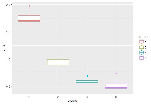
It was not possible to check on 16 streams, but it is clear that when going from 1 to 4 streams, the speed increases about three times, which is very pleasing.

4. reticulate and iterators

To work with data that does not fit in memory, we use iterators from the reticulate package. The basis is a normal closure function (ie, a function that, when called, returns another function along with the call environment:

 train_generator <- function(images_dir, samples_index, masks_dir, batch_size) { images_iter <- list.files(images_dir, pattern = ".jpg", full.names = TRUE)[samples_index] # for current epoch images_all <- list.files(images_dir, pattern = ".jpg", full.names = TRUE)[samples_index] # for next epoch masks_iter <- list.files(masks_dir, pattern = ".gif", full.names = TRUE)[samples_index] # for current epoch masks_all <- list.files(masks_dir, pattern = ".gif", full.names = TRUE)[samples_index] # for next epoch function() { # start new epoch if (length(images_iter) < batch_size) { images_iter <<- images_all masks_iter <<- masks_all } batch_ind <- sample(1:length(images_iter), batch_size) batch_images_list <- images_iter[batch_ind] images_iter <<- images_iter[-batch_ind] batch_masks_list <- masks_iter[batch_ind] masks_iter <<- masks_iter[-batch_ind] x_y_batch <- foreach(i = 1:batch_size) %dopar% { x_y_imgs <- imagesRead(image_file = batch_images_list[i], mask_file = batch_masks_list[i]) # augmentation x_y_imgs$img <- randomBSH(x_y_imgs$img) x_y_imgs <- randomHorizontalFlip(x_y_imgs$img, x_y_imgs$mask) # return as arrays x_y_arr <- list(x = img2arr(x_y_imgs$img), y = mask2arr(x_y_imgs$mask)) } x_y_batch <- purrr::transpose(x_y_batch) x_batch <- do.call(abind, c(x_y_batch$x, list(along = 1))) y_batch <- do.call(abind, c(x_y_batch$y, list(along = 1))) result <- list(keras_array(x_batch), keras_array(y_batch)) return(result) } } 

 val_generator <- function(images_dir, samples_index, masks_dir, batch_size) { images_iter <- list.files(images_dir, pattern = ".jpg", full.names = TRUE)[samples_index] # for current epoch images_all <- list.files(images_dir, pattern = ".jpg", full.names = TRUE)[samples_index] # for next epoch masks_iter <- list.files(masks_dir, pattern = ".gif", full.names = TRUE)[samples_index] # for current epoch masks_all <- list.files(masks_dir, pattern = "gif", full.names = TRUE)[samples_index] # for next epoch function() { # start new epoch if (length(images_iter) < batch_size) { images_iter <<- images_all masks_iter <<- masks_all } batch_ind <- sample(1:length(images_iter), batch_size) batch_images_list <- images_iter[batch_ind] images_iter <<- images_iter[-batch_ind] batch_masks_list <- masks_iter[batch_ind] masks_iter <<- masks_iter[-batch_ind] x_y_batch <- foreach(i = 1:batch_size) %dopar% { x_y_imgs <- imagesRead(image_file = batch_images_list[i], mask_file = batch_masks_list[i]) # without augmentation # return as arrays x_y_arr <- list(x = img2arr(x_y_imgs$img), y = mask2arr(x_y_imgs$mask)) } x_y_batch <- purrr::transpose(x_y_batch) x_batch <- do.call(abind, c(x_y_batch$x, list(along = 1))) y_batch <- do.call(abind, c(x_y_batch$y, list(along = 1))) result <- list(keras_array(x_batch), keras_array(y_batch)) return(result) } } 

Here, in the call environment, lists of processed files are decreasing during each epoch, as well as copies of complete lists that are used at the beginning of each next epoch. In this implementation, there is no need to worry about randomly mixing files - each batch is obtained by random sampling.

As shown above, x_y_batch is a list of 16 lists, each of which is a list of 2 arrays. The function purrr::transpose() turns the nested lists inside out, and we get a list of 2 lists, each of which is a list of 16 arrays. abind() joins arrays along the specified dimension, do.call() passes an arbitrary number of arguments to the internal function. Additional arguments ( along = 1 ) are specified in a rather bizarre way: do.call(abind, c(x_y_batch$x, list(along = 1))) .

It remains to turn these functions into objects that are understandable for Keras , using py_iterator() :

 train_iterator <- py_iterator(train_generator(images_dir = images_dir, masks_dir = masks_dir, samples_index = train_index, batch_size = batch_size)) val_iterator <- py_iterator(val_generator(images_dir = images_dir, masks_dir = masks_dir, samples_index = val_index, batch_size = batch_size)) 

Calling iter_next(train_iterator) will return the result of performing one iteration, which is useful at the debugging stage.

5. The segmentation task and the loss function for it

The segmentation task can be considered as pixel-by-pixel classification: each pixel is predicted to belong to a particular class. For the case of two classes, the result will be a mask; if there are more than two classes, the number of masks will be equal to the number of classes minus 1 (analogous to one-hot encodind). There are only two classes in our competition (the machine and the background), the quality metric is the dice-factor . He calculates as follows:

 K <- backend() dice_coef <- function(y_true, y_pred, smooth = 1.0) { y_true_f <- K$flatten(y_true) y_pred_f <- K$flatten(y_pred) intersection <- K$sum(y_true_f * y_pred_f) result <- (2 * intersection + smooth) / (K$sum(y_true_f) + K$sum(y_pred_f) + smooth) return(result) } 

We will optimize the loss function, which is the sum of the cross-entropy and 1 - dice_coef :

 bce_dice_loss <- function(y_true, y_pred) { result <- loss_binary_crossentropy(y_true, y_pred) + (1 - dice_coef(y_true, y_pred)) return(result) } 

6. U-Net architecture

U-Net is a classic architecture for solving segmentation problems. Schematic diagram:

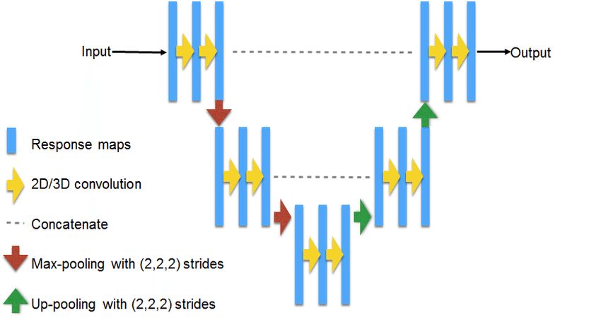
Source: https://www.researchgate.net/figure/311715357_fig3_Fig-3-U-NET-Architecture

Implementation for pictures 128x128:

 get_unet_128 <- function(input_shape = c(128, 128, 3), num_classes = 1) { inputs <- layer_input(shape = input_shape) # 128 down1 <- inputs %>% layer_conv_2d(filters = 64, kernel_size = c(3, 3), padding = "same") %>% layer_batch_normalization() %>% layer_activation("relu") %>% layer_conv_2d(filters = 64, kernel_size = c(3, 3), padding = "same") %>% layer_batch_normalization() %>% layer_activation("relu") down1_pool <- down1 %>% layer_max_pooling_2d(pool_size = c(2, 2), strides = c(2, 2)) # 64 down2 <- down1_pool %>% layer_conv_2d(filters = 128, kernel_size = c(3, 3), padding = "same") %>% layer_batch_normalization() %>% layer_activation("relu") %>% layer_conv_2d(filters = 128, kernel_size = c(3, 3), padding = "same") %>% layer_batch_normalization() %>% layer_activation("relu") down2_pool <- down2 %>% layer_max_pooling_2d(pool_size = c(2, 2), strides = c(2, 2)) # 32 down3 <- down2_pool %>% layer_conv_2d(filters = 256, kernel_size = c(3, 3), padding = "same") %>% layer_batch_normalization() %>% layer_activation("relu") %>% layer_conv_2d(filters = 256, kernel_size = c(3, 3), padding = "same") %>% layer_batch_normalization() %>% layer_activation("relu") down3_pool <- down3 %>% layer_max_pooling_2d(pool_size = c(2, 2), strides = c(2, 2)) # 16 down4 <- down3_pool %>% layer_conv_2d(filters = 512, kernel_size = c(3, 3), padding = "same") %>% layer_batch_normalization() %>% layer_activation("relu") %>% layer_conv_2d(filters = 512, kernel_size = c(3, 3), padding = "same") %>% layer_batch_normalization() %>% layer_activation("relu") down4_pool <- down4 %>% layer_max_pooling_2d(pool_size = c(2, 2), strides = c(2, 2)) # 8 center <- down4_pool %>% layer_conv_2d(filters = 1024, kernel_size = c(3, 3), padding = "same") %>% layer_batch_normalization() %>% layer_activation("relu") %>% layer_conv_2d(filters = 1024, kernel_size = c(3, 3), padding = "same") %>% layer_batch_normalization() %>% layer_activation("relu") # center up4 <- center %>% layer_upsampling_2d(size = c(2, 2)) %>% {layer_concatenate(inputs = list(down4, .), axis = 3)} %>% layer_conv_2d(filters = 512, kernel_size = c(3, 3), padding = "same") %>% layer_batch_normalization() %>% layer_activation("relu") %>% layer_conv_2d(filters = 512, kernel_size = c(3, 3), padding = "same") %>% layer_batch_normalization() %>% layer_activation("relu") %>% layer_conv_2d(filters = 512, kernel_size = c(3, 3), padding = "same") %>% layer_batch_normalization() %>% layer_activation("relu") # 16 up3 <- up4 %>% layer_upsampling_2d(size = c(2, 2)) %>% {layer_concatenate(inputs = list(down3, .), axis = 3)} %>% layer_conv_2d(filters = 256, kernel_size = c(3, 3), padding = "same") %>% layer_batch_normalization() %>% layer_activation("relu") %>% layer_conv_2d(filters = 256, kernel_size = c(3, 3), padding = "same") %>% layer_batch_normalization() %>% layer_activation("relu") %>% layer_conv_2d(filters = 256, kernel_size = c(3, 3), padding = "same") %>% layer_batch_normalization() %>% layer_activation("relu") # 32 up2 <- up3 %>% layer_upsampling_2d(size = c(2, 2)) %>% {layer_concatenate(inputs = list(down2, .), axis = 3)} %>% layer_conv_2d(filters = 128, kernel_size = c(3, 3), padding = "same") %>% layer_batch_normalization() %>% layer_activation("relu") %>% layer_conv_2d(filters = 128, kernel_size = c(3, 3), padding = "same") %>% layer_batch_normalization() %>% layer_activation("relu") %>% layer_conv_2d(filters = 128, kernel_size = c(3, 3), padding = "same") %>% layer_batch_normalization() %>% layer_activation("relu") # 64 up1 <- up2 %>% layer_upsampling_2d(size = c(2, 2)) %>% {layer_concatenate(inputs = list(down1, .), axis = 3)} %>% layer_conv_2d(filters = 64, kernel_size = c(3, 3), padding = "same") %>% layer_batch_normalization() %>% layer_activation("relu") %>% layer_conv_2d(filters = 64, kernel_size = c(3, 3), padding = "same") %>% layer_batch_normalization() %>% layer_activation("relu") %>% layer_conv_2d(filters = 64, kernel_size = c(3, 3), padding = "same") %>% layer_batch_normalization() %>% layer_activation("relu") # 128 classify <- layer_conv_2d(up1, filters = num_classes, kernel_size = c(1, 1), activation = "sigmoid") model <- keras_model( inputs = inputs, outputs = classify ) model %>% compile( optimizer = optimizer_rmsprop(lr = 0.0001), loss = bce_dice_loss, metrics = c(dice_coef) ) return(model) } model <- get_unet_128() 

The curly braces in {layer_concatenate(inputs = list(down4, .), axis = 3)} are needed to substitute the object as the desired argument, and not as the first in a row, as the %>% operator would otherwise do. You can offer many modifications of this architecture: use layer_conv_2d_transpose instead of layer_upsampling_2d , apply separate convolutions of layer_separable_conv_2d instead of usual ones, experiment with filter numbers and with optimizers settings. Under the link Kaggle Carvana Image Masking Challenge solution with Keras there are options for resolutions up to 1024x1024, which are also easily ported to R.

There are a lot of parameters in our model:

 # Total params: 34,540,737 # Trainable params: 34,527,041 # Non-trainable params: 13,696 

7. Model training

It's simple. Run the Tensorboard:

 tensorboard("logs_r") 

Alternatively, the tfruns package is available , which adds an analogue of Tensorboard to the RStudio IDE and allows you to streamline the work of training neural networks.

Specify the callback. We will use the early stop, reduce the speed of learning when reaching the plateau and save the weight of the best model:

 callbacks_list <- list( callback_tensorboard("logs_r"), callback_early_stopping(monitor = "val_python_function", min_delta = 1e-4, patience = 8, verbose = 1, mode = "max"), callback_reduce_lr_on_plateau(monitor = "val_python_function", factor = 0.1, patience = 4, verbose = 1, epsilon = 1e-4, mode = "max"), callback_model_checkpoint(filepath = "weights_r/unet128_{epoch:02d}.h5", monitor = "val_python_function", save_best_only = TRUE, save_weights_only = TRUE, mode = "max" ) ) 

We start training and we wait. On the GTX 1050ti, one era takes about 10 minutes:

 model %>% fit_generator( train_iterator, steps_per_epoch = as.integer(length(train_index) / batch_size), epochs = epochs, validation_data = val_iterator, validation_steps = as.integer(length(val_index) / batch_size), verbose = 1, callbacks = callbacks_list ) 

8. Model Predictions

- run-length encoding.

 test_dir <- "input/test/" test_samples <- 100064 test_index <- sample(1:test_samples, 1000) load_model_weights_hdf5(model, "weights_r/unet128_08.h5") # best model imageRead <- function(image_file, target_width = 128, target_height = 128) { img <- image_read(image_file) img <- image_scale(img, paste0(target_width, "x", target_height, "!")) } img2arr <- function(image, target_width = 128, target_height = 128) { result <- aperm(as.numeric(image[[1]])[, , 1:3], c(2, 1, 3)) # transpose dim(result) <- c(1, target_width, target_height, 3) return(result) } arr2img <- function(arr, target_width = 1918, target_height = 1280) { img <- image_read(arr) img <- image_scale(img, paste0(target_width, "x", target_height, "!")) } qrle <- function(mask) { img <- t(mask) dim(img) <- c(128, 128, 1) img <- arr2img(img) arr <- as.numeric(img[[1]])[, , 2] vect <- ifelse(as.vector(arr) >= 0.5, 1, 0) turnpoints <- c(vect, 0) - c(0, vect) starts <- which(turnpoints == 1) ends <- which(turnpoints == -1) paste(c(rbind(starts, ends - starts)), collapse = " ") } cl <- makePSOCKcluster(4) clusterEvalQ(cl, { library(magick) library(abind) library(reticulate) imageRead <- function(image_file, target_width = 128, target_height = 128) { img <- image_read(image_file) img <- image_scale(img, paste0(target_width, "x", target_height, "!")) } img2arr <- function(image, target_width = 128, target_height = 128) { result <- aperm(as.numeric(image[[1]])[, , 1:3], c(2, 1, 3)) # transpose dim(result) <- c(1, target_width, target_height, 3) return(result) } qrle <- function(mask) { img <- t(mask) dim(img) <- c(128, 128, 1) img <- arr2img(img) arr <- as.numeric(img[[1]])[, , 2] vect <- ifelse(as.vector(arr) >= 0.5, 1, 0) turnpoints <- c(vect, 0) - c(0, vect) starts <- which(turnpoints == 1) ends <- which(turnpoints == -1) paste(c(rbind(starts, ends - starts)), collapse = " ") } }) registerDoParallel(cl) test_generator <- function(images_dir, samples_index, batch_size) { images_iter <- list.files(images_dir, pattern = ".jpg", full.names = TRUE)[samples_index] function() { batch_ind <- sample(1:length(images_iter), batch_size) batch_images_list <- images_iter[batch_ind] images_iter <<- images_iter[-batch_ind] x_batch <- foreach(i = 1:batch_size) %dopar% { img <- imageRead(image_file = batch_images_list[i]) # return as array arr <- img2arr(img) } x_batch <- do.call(abind, c(x_batch, list(along = 1))) result <- list(keras_array(x_batch)) } } test_iterator <- py_iterator(test_generator(images_dir = test_dir, samples_index = test_index, batch_size = batch_size)) preds <- predict_generator(model, test_iterator, steps = 10) preds <- foreach(i = 1:160) %dopar% { result <- qrle(preds[i, , , ]) } preds <- do.call(rbind, preds) 

, qrle , ( skoffer -):

results

:

— 128128. , , .

, .

Total
In this message, it was shown that, while sitting on R, one can keep up with fashion trends and successfully train deep neural networks. And even the Windows OS is not able to prevent this.
Continuation, as usual, follows.