Change sex and race on a selfie using neural networks

Hi, Habr! Today I want to tell you how you can change your face in the photo, using a rather complex pipeline from several generative neural networks and not only. Recently fashionable applications for transforming oneself into a lady or grandfather work easier, because neural networks are slow, and the quality that can be obtained by classical methods of computer vision is already good. Nevertheless, the proposed method seems to me very promising. Under the cut there will be little code, but a lot of pictures, links and personal experience with GANs.

The task can be divided into the following steps:

• find and cut the face in the photo
• convert the face as necessary (turn into a woman / black, etc.)
• improve / enlarge the resulting image
• paste the transformed face back into the original photo

Each of these steps can be implemented as a separate neural network, but you can do without them. Let's take it in order.

Face detection

Here is the easiest. You can not invent anything and just take dlib.get_frontal_face_detector() ( example ). Dlib's default detector uses a linear classifier trained on HOG features.

As we can see, the issued rectangle does not contain the entire face, so it’s better to enlarge it. Optimum zoom factors can be hand picked. As a result, you can get a similar method and a similar result:

 def detect_single_face_dlib(img_rgb, rescale=(1.1, 1.5, 1.1, 1.3)): fd_front_dlib = dlib.get_frontal_face_detector() face = fd_front_dlib(img_rgb, 1) if len(face) > 0: face = sorted([(t.width() * t.height(), (t.left(), t.top(), t.width(), t.height())) for t in face], key=lambda t: t[0], reverse=True)[0][1] else: return None if rescale is not None and face is not None: if type(rescale) != tuple: rescale = (rescale, rescale, rescale, rescale) (x, y, w, h) = face w = min(img_rgb.shape[1] - x, int(w / 2 + rescale[2] * w / 2)) h = min(img_rgb.shape[0] - y, int(h / 2 + rescale[3] * h / 2)) fx = max(0, int(x + w / 2 * (1 - rescale[0]))) fy = max(0, int(y + h / 2 * (1 - rescale[1]))) fw = min(img_rgb.shape[1] - fx, int(w - w / 2 * (1 - rescale[0]))) fh = min(img_rgb.shape[0] - fy, int(h - h / 2 * (1 - rescale[1]))) face = (fx, fy, fw, fh) return face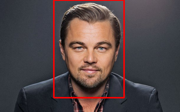 

If the work of the "old" methods for some reason does not suit you, you can try deep learning. To solve the problem of face detection, any Region Proposal Networks will suit, for example, YOLOv2 or Faster-RCNN . How to try - be sure to share what you got.

Face transformation

Here is the most interesting. As you probably already know , you can transform a face or make a mask without neural networks, and it will work well. But generative networks are a much more promising tool for image processing. There are already a huge number of models, such as <your prefix>GAN , that can do a variety of transformations. The task of converting images from one set (domain) to another is called Domain Transfer. You could get acquainted with some Domain Transfer architectures in our recent review of GANs .

Cycle-gan

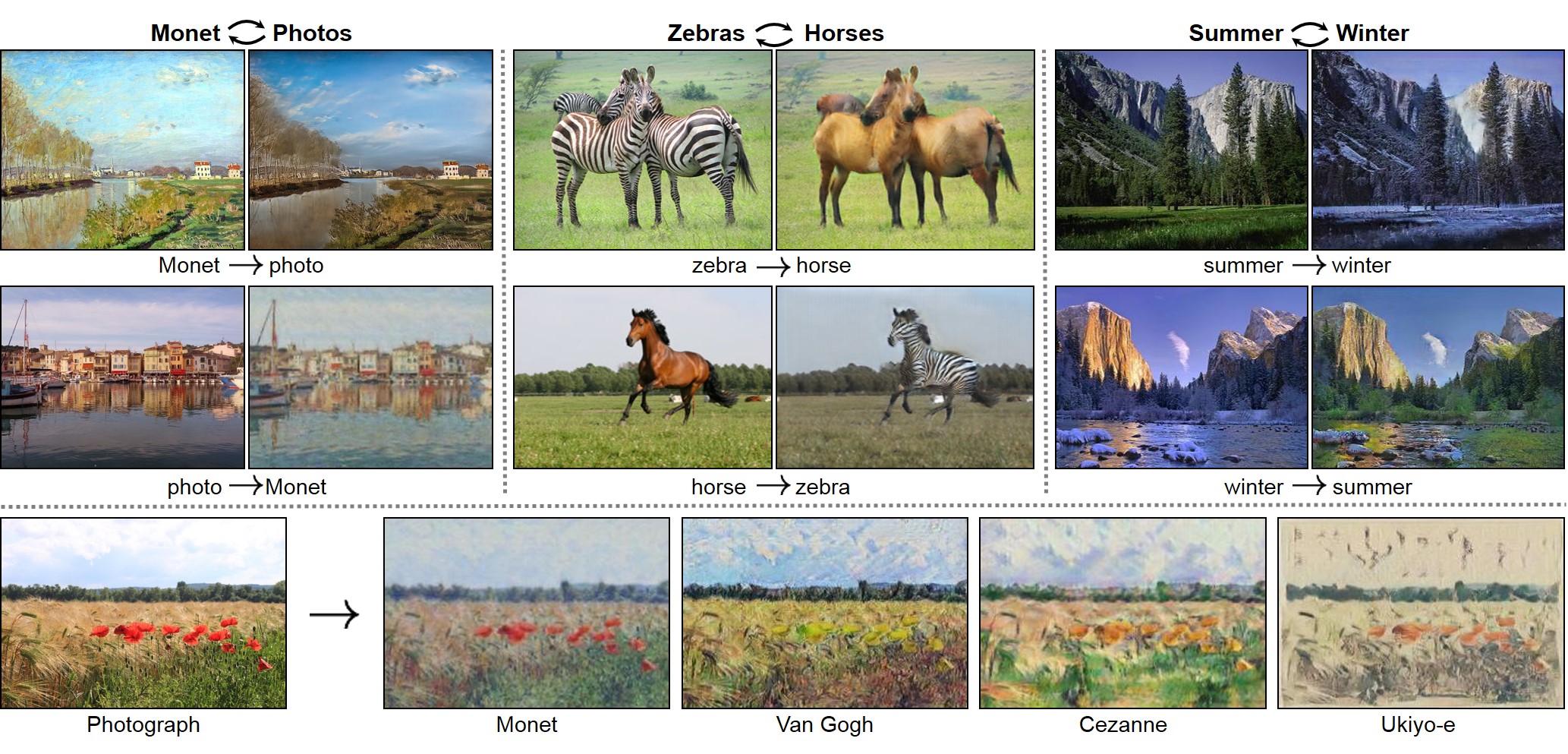
Why choose Cycle-GAN? Yes, because it works. Visit the project site and see what you can do with this model. As a dataset, two sets of images are enough: DomainA and DomainB. Let's say you have folders with photos of men and women, whites and Asians, apples and peaches. It's enough! Clone the author's repository with the implementation of Cycle-GAN on pytorch and start learning.

How it works

In this figure from the original article, the principle of the model operation is described quite fully and briefly. In my opinion, a very simple and elegant solution that gives good results.

In fact, we train two generator functions. One - $$$G$ - learns from the input image from the domain $$$X$ generate image from domain $$$Y$ . Other - $$$F$ - on the contrary, from $$$Y$ at $$$X$ . Relevant discriminators $$$D_Y$ and $$$D_x$ they are helped in this, as is characteristic of the GANs. A typical Advesarial Loss (or GAN Loss) looks like this:

Additionally, the authors introduce the so-called Cycle Consistensy Loss:

Its essence is to image from the domain $$$X$ after going through a generator $$$G$ and then through the generator $$$F$ It was most similar to the original. In short $$$F (G (x)) \ approx x$ .

Thus, the objective function takes the form:

and we solve the following optimization problem:

Here $$$\ lambda$ - a hyperparameter controlling the weight of the extra loss.

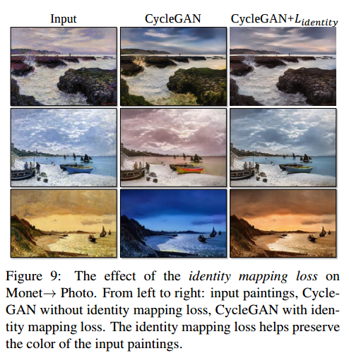
But that is not all. It was noticed that the generators greatly change the color gamut of the original image.

To fix this, the authors added an additional loss - Identity Loss. This is a kind of regularizer that requires identity mapping from the generator for images of the target domain. Those. if a zebra came to the zebra generator, then you don’t need to change such a picture.

To (my) surprise, this helped solve the problem of preserving colors. Here are examples from the authors of the article (Monet’s paintings are trying to be converted into real photos):

Network Architecture

In order to describe the used architecture, we introduce some conventions.

c7s1-k is a 7x7 convolutional layer followed by a batch normalization and ReLU, with Straight 1, Padding 3 and the number of filters k. Such layers do not reduce the dimension of our image. Example on pytorch:

 [nn.Conv2d(n_channels, inplanes, kernel_size=7, padding=3), nn.BatchNorm2d(k, affine=True), nn.ReLU(True)] 

dk - 3x3 convolutional layer with a stride 2 and the number of filters k. Such convolutions reduce the dimension of the input image by 2 times. Again the pytorch example:

 [nn.Conv2d(inplanes, inplanes * 2, kernel_size=3, stride=2, padding=1), nn.BatchNorm2d(inplanes * 2, affine=True), nn.ReLU(True)] 

Rk - residual block with two 3x3 convolutions with the same number of filters. The authors, it is designed as follows:

 resnet_block = [] resnet_block += [nn.Conv2d(inplanes, planes, kernel_size=3, stride=1, padding=1), nn.BatchNorm2d(planes, affine=True), nn.ReLU(inplace=True)] resnet_block += [nn.Conv2d(planes, planes, kernel_size=3, stride=1, padding=1), nn.BatchNorm2d(planes, affine=True)] 

uk - 3x3 up-convolution layer with BatchNorm and ReLU - to increase image dimension. Again an example:

 [nn.ConvTranspose2d(inplanes * 4, inplanes * 2, kernel_size=3, stride=2, padding=1, output_padding=1), nn.BatchNorm2d(inplanes * 2, affine=True), nn.ReLU(True)] 

With the above designations, a generator with 9 reznet-blocks looks like this:

c7s1-32,d64,d128,R128,R128,R128,R128,R128,R128,R128,R128,R128,u64,u32,c7s1-3

We do the initial convolution with 32 filters, then reduce the image twice, simultaneously increasing the number of filters, then go 9 reznet-blocks, then twice increasing the image, reducing the number of filters, and creating a final 3-channel output of our neural network.

For the discriminator, we will use the notation Ck - 4x4 convolution followed by a batch-norm and LeakyReLU with parameter 0.2. The discriminator architecture is as follows:

C64-C128-C256-C512

In this case, for the first layer of C64 we do not do BatchNorm.

And at the end we add one neuron with a sigmoid activation function, which says whether it has come to fake or not.

Just a few words about the discriminator

Such a discriminator is the so-called fully-convolutional network - there are no fully connected layers, only convolution. Such networks can receive images of any size as input, and the number of layers controls the receptive field of the network. For the first time such an architecture was presented in the Fully Convolutional Networks for Semantic Segmentation article.

In our case, the generator mapping the input image is not on one scalar, as usual, but on 512 output images (of reduced size), which are used to draw the "real or fake" output. This can be interpreted as a weighted vote on 512 patches of the input image. The size of the patch (receptive field) can be estimated by forwarding all activations back to the input. But good people made a utility that considers everything for us. Such networks are also called PatchGAN.

In our case, the 3-layer PatchGAN with an input image of 256x256 has a receptive field of 70x70, and this is equivalent to how we would cut out a few random patches of 70x70 from the input and judged by it, the actual picture came or generated. By controlling the depth of the network, we can control the size of the patches. For example, a 1-layer PatchGAN has a 16x16 receptive field, and in this case we are looking at low-level features. 5-layer PatchGAN will already look at almost the entire picture. Here Phillip Isola clearly explained all this magic to me. Read, you too should become clearer. The main thing: fully convolutional networks work better than usual, and they should be used.

Features of learning Cycle-GAN

Data

To begin with, we tried to solve the problem of transforming the faces of men into women and vice versa. The blessing, for this purpose is. For example, CelebA , containing 200 thousand photos of celebrities with binary marks Gender, Points, Beard, etc.

Actually, having broken this dataset by the necessary attribute, we get about 90k pictures of men and 110k - women. These are our DomainX and DomainY.

However, the average size of the faces on these photos is not very large (about 150x150), and instead of resizing all the images to 256x256, we brought them to 128x128. Also, to preserve the aspect ratio, the pictures did not stretch, but fit into the black square 128x128. A typical generator input might look like this:

Perceptual Loss

Intuition and experience prompted us to consider identity loss not in the pixel space, but in the feature space of the pre-trained VGG-16 network. This is the trick that was first introduced in the article Perceptual Losses for Real-Time Style Transfer and Super-Resolution and is widely used in Style Transfer tasks. The logic here is simple: if we want to make generators invariant to the style of images from the target domain, then why consider the error on pixels, if there are features containing style information. What effect this has led you will find out a little later.

Learning procedure

In general, the model was quite cumbersome, 4 networks are studying right away. Images on them should be driven back and forth several times to calculate all the losses, and then spread back all the gradients. One epoch of learning at CelebA (200k pictures 128x128) on GForce 1080 takes about 5 hours. So do not particularly experiment. Let me just say that our configuration differed from the author only by replacing Identity Loss with Perceptual. PatchGANs with more or fewer layers did not go, left 3-ply. Optimizer for all networks - Adam with parameters betas=(0.5, 0.999) . The learning rate defaults to 0.0002 and decreases each epoch. BatchSize was equal to 1, and in all grids BatchNorm was replaced (by the authors) with InstanceNorm. An interesting point is that the input to the discriminator was not the last output of the generator, but a random picture from the buffer of 50 images. Thus, the discriminator could come image generated by the previous version of the generator. This trick and many others that the authors used are listed in the Sumit Chintala note (by PyTorch) How to Train a GAN? Tips and tricks to make GANs work . I recommend to print this list and hang it near the workplace. We did not reach out to try everything that is there, for example, LeakyReLU and alternative methods of upsampling for the generator. But they fiddled with the discriminator and training schedule of the generator / discriminator pair. It really adds stability.

Experiments

Now will go more pictures, you probably already waited.

In general, learning of generative networks is somewhat different from other tasks of deep learning. Here you often will not see your usual picture of the downward-losing and growing metrics of quality. Rate how good your model can only be looking at the outputs of the generators. A typical picture that we saw looked like this:

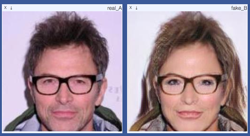
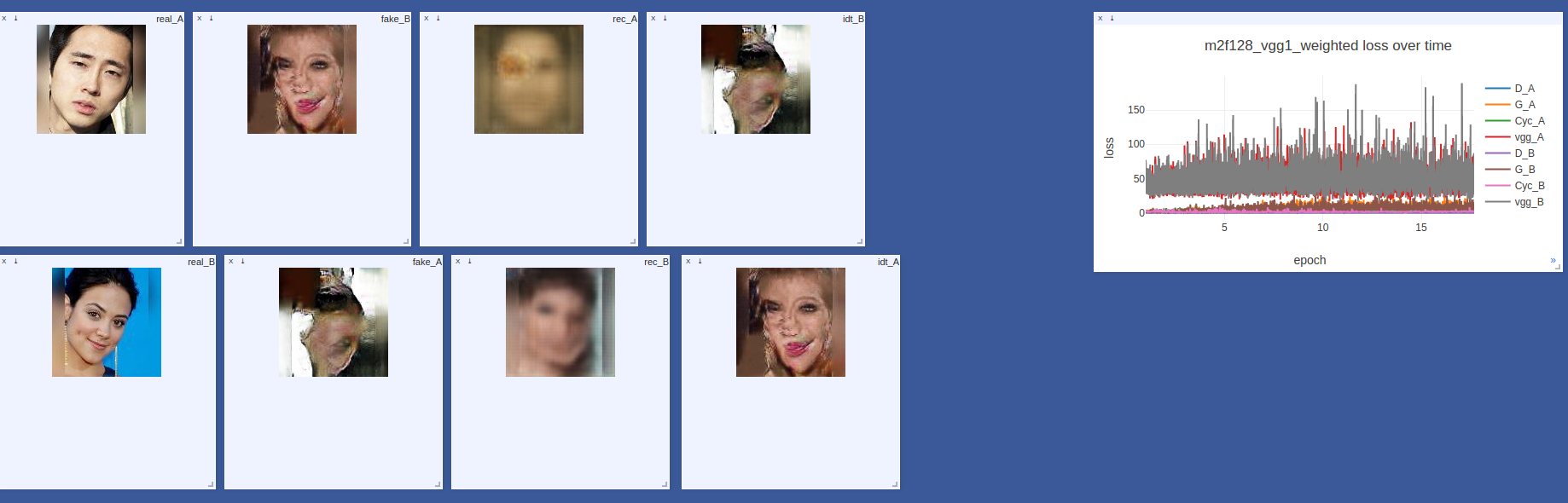
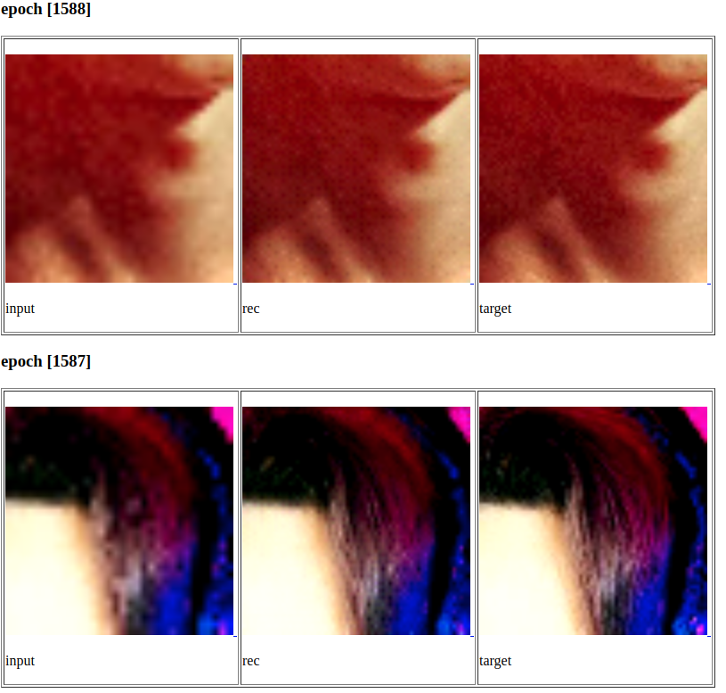
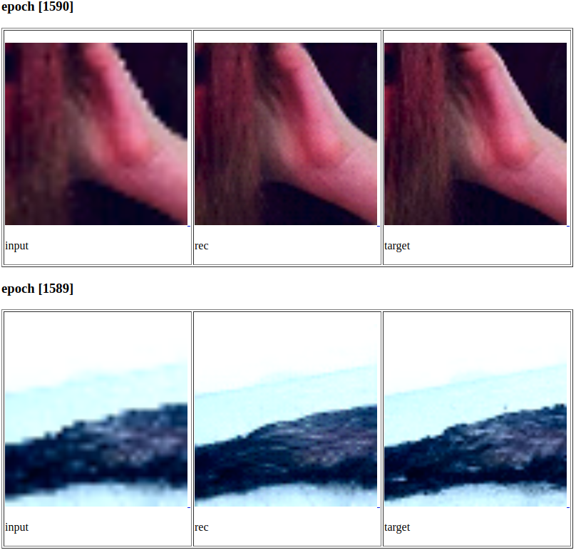
The generators gradually disperse, the other Losses slightly decreased, but nevertheless, the network produces decent pictures and obviously learned something. By the way, we used visdom , a fairly easy to set up and handy tool from Facebook Research, to visualize the course of the model. Every few iterations we looked at the following 8 pictures:

• real_A - login from domain A
• fake_B - real_A, converted by generator A-> B
• rec_A - reconstructed image, fake_B, converted by generator B-> A
• idty_B - real_A, converted by generator B-> A
• and 4 similar images on the reverse side

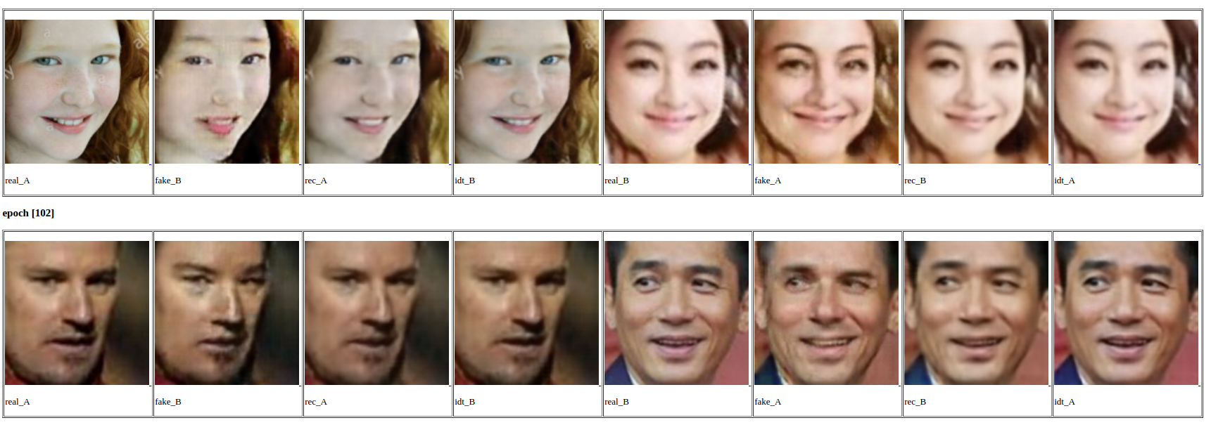
In average, good results can be seen after the 5th era of training. Look, the error of the generators does not decrease in any way, but this did not prevent the network from turning a person like Hinton into a woman. Nothing holy!

Sometimes things can go really bad.

In this case, you can press Ctrl + C and call journalists, tell how you stopped artificial intelligence.

In general, despite some artifacts and low resolution, Cycle-GAN with a bang coped with the task.

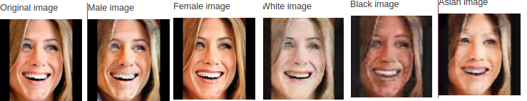
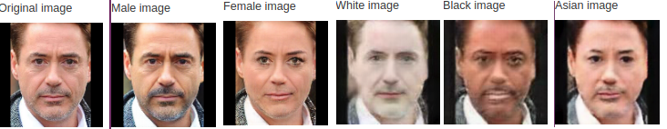
See for yourself:

Men <-> Women

White <-> Asians

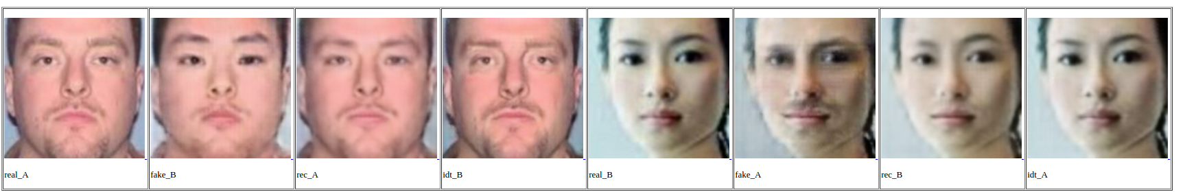
White <-> Black

Have you noticed the interesting effect that identity mapping and perceptual loss give? Look at idty_A and idty_B. A woman becomes more feminine (more make-up, smooth, light skin), a man gets facial hair, whites become even whiter, and black, correspondingly, blacker. Generators learn the average style for the entire domain, thanks to perceptual loss. This is where the creation of an application for the "beautification" of your photos is directly suggested. Shut up and give me your money!

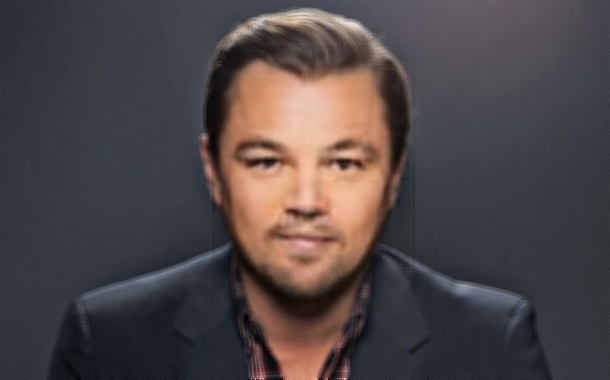
Here is Leo:

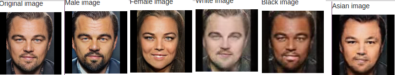
And a few more celebrities:

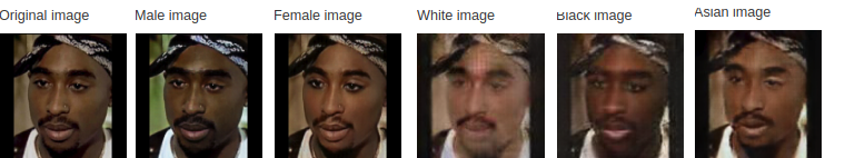
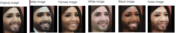
Personally, this guy-Jolie scared me.

And now, attention, a very complicated case.

Increase resolution

CycleGAN coped well with the task. But the resulting images are of small size and some artifacts. The task of increasing the resolution is called Image Superresolution. And we have already learned how to solve this problem using neural networks. I want to mention two state-of-the-art models: SR-ResNet and EDSR.

SRResNet

In the article " A Generative Adversarial Network", the authors propose a generation network architecture for the super-resolution task (SRGAN), which is based on ResNet. In addition to the pixel-based MSE, the authors add Perceptual loss using activations from the pre-trained VGG (see, everyone does it!) And the discriminator, naturally.

The generator uses residual blocks with 3x3 convolutions, 64 filters, batchnorm and ParametricReLu. Two subPixel layers are used to increase the resolution.

The discriminator has 8 convolutional layers with a 3x3 core and an increasing number of channels from 64 to 512, activation everywhere is LeakyReLu, after each doubling of the number of features, the image resolution decreases due to stride in convolutions. There are no pooling layers; at the end, two fully connected layers and a sigmoid for classification. A schematic of the generator and discriminator is shown below.

EDSR

Enhanced Deep Super-Resolution network is the same SRResNet, but with three modifications:

• No batch normalization. This allows reducing up to 40% of the memory used during training and increasing the number of filters and layers
• Outside residual blocks not used ReLu
• all resnet blocks are multiplied by a factor of 0.1 before adding them to previous activations. This allows you to stabilize learning.

Training

To learn the SR network, you need to have high resolution datsets. Some effort and time had to be spent on parsing several thousand photos from instagram on the #face hashtag. But where without it, we all know that the collection and processing of data is 80 +% of the volume of our work.

Teaching the SR network is not made on full images, but on small patches cut from them. This allows the generator to learn how to work with small parts. And in the working mode, the input of the network can be submitted images of any size, because this is a fully-convolutional network.

In practice, the EDSR, which supposedly should work better and faster than its predecessor SRResNet, did not show the best results and studied much slower.

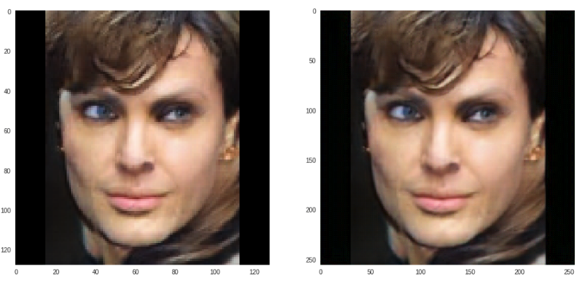
As a result, we chose SRRestNet, trained on 64x64 patches, for our Peripual loss 2 and 5 layers of VGG-16 were used, and we generally removed the discriminator. Below are a few examples from the training set.

And this is how this model works on our artificial images. Not ideal, but not bad.

Insert image in original

Even this task can be solved by neural networks. I found one interesting job on image blending. GP-GAN: Towards Realistic High-Resolution Image Blending . I will not tell the details, I will show only a picture from the article.

We did not have time to implement this thing, we got off with a simple solution. We insert our square with the transformed face back into the original, gradually increasing the transparency of the image closer to the edges. It turns out like this:

Again, not ideal, but in haste - ok.

Conclusion

Many things can still be tried to improve the current result. I have a whole list, I just need time and more video cards.

And in general, I really want to get together on some hackathon and finish the resulting prototype to a normal web application.

And then you can think about trying to transfer Ghana to mobile devices. To do this, you need to try different techniques to accelerate and reduce neural networks: factorization, knowledge distillation, that's all. And about this we will soon have a separate post, stay tuned. See you again!