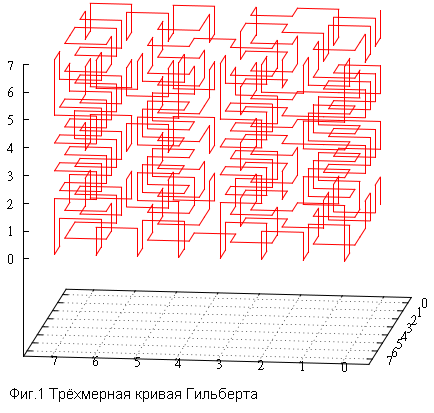
Hilbert curve vs Z-order

I have repeatedly heard the opinion that of all sweeping curves . It is the Hilbert curve that is most promising for spatial indexing. It is motivated by the fact that it does not contain discontinuities and therefore, in a sense, is “well-arranged.” Is this so in reality and what does spatial indexing mean here, let's figure it out under the cat.

The final article from the cycle:

• Why does not the rectilinear approach work when
  spatial indexing by sweeping curves
• Algorithm Presentation
• 3D and obvious optimizations
• 8D and prospects in OLAP
• 3D on the sphere, what it looks like
• 3D sphere, benchmarks
• How about indexing non-point objects?

The Hilbert curve has a remarkable property - the distance between two consecutive points on it is always equal to one (the current detail step, more precisely). Therefore, the data with not very different values ​​of the Hilbert curve are located close to each other (the opposite, by the way, is wrong - the neighboring points of Moget differ greatly in meaning). For the sake of this property it is used, for example, for

• downscaling ( color palette management )
• increase locality of access in multidimensional indexing ( here )
• in antenna construction ( here )
• table clustering ( DB2 )

As for spatial data, the properties of the Hilbert curve allow to increase the locality of links and improve the efficiency of the database cache, as here , where before using the table it is recommended to supplement it with a column with the calculated value and sort by this column.
')
In spatial search, the Hilbert curve is present in Hilbert R-trees , where the main idea (very roughly) - when it comes time to split a page into two descendants - we sort all the elements on the page by centroid values ​​and divide in half.

But we are more interested in another property of the Hilbert curve — it is a self-similar sweeping curve. That allows to use it in an index on the basis of the B-tree. We are talking about the method of numbering the discrete space.

• Let a discrete space of dimension N be given.
• Suppose also that we have some way of numbering all points of this space.
• Then, for indexing point objects, it is enough to place in the index on the basis of the B-tree the numbers of points to which these objects fall.
• Search in such a spatial index depends on the method of numbering and ultimately comes down to a sample by index from the ranges of values.
• Sweeping curves are good for their self-similarity, which allows for the generation of a relatively small number of such subintervals, while other methods (for example, a similarity of the lower-case scanning) require a huge number of subqueries, which makes such spatial indexing ineffective.
  

So where does this intuitive feeling come from, that the Hilbert curve is good for spatial indexing? Yes, there are no gaps in it, the distance between any consecutive points is equal to the sampling step. So what? What is the relationship between this fact and potentially high performance?

At the very beginning, we formulated a rule - a “good” numbering method minimizes the total perimeter of index pages. We are talking about the pages of the B-tree, on which data will eventually appear. In other words, index performance is determined by the number of pages to read. The smaller pages on average for a query of the reference size, the higher the (potential) index performance.

From this point of view, the Hilbert curve looks very promising. But this intuitive sensation cannot be smeared on bread, so we will conduct a numerical experiment.

• consider 2 and 3-dimensional spaces
• take square / cubic requests of different sizes
• for a series of random queries of the same type and size, we calculate the average / variance of the number of visible pages in a series of 1000 queries
• let us proceed from the fact that there is a point at each node of space. You can jot down random data and check for it, but then there would be questions about the quality of this random data. And so we have a completely objective indicator of “suitability”, albeit far from any real data set.
• 200 elements are placed on the page, it is important that this would not be a power of two, which would lead to a degenerate case
• compare the Hilbert curve and the Z-curve

This is how it looks like graphs.



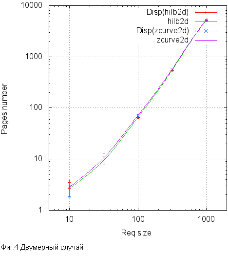
Now it is worth at least out of curiosity to see how with a fixed request size (2D 100X100) the number of read pages behaves, depending on the page size.


The “pits” in the Z-order are well visible, corresponding to sizes 128, 256 and 512. And there are “pits” in 192, 384, 768. Not so big.

As we can see, the difference can reach 10%, but almost everywhere it is within the statistical error. Nevertheless, the Hilbert curve everywhere behaves better than the Z-curve. Not much, but better. Apparently, this 10% is the upper estimate of the potential effect that can be achieved by switching to the Hilbert curve. Is the game worth the candle? Let's try to find out.

Implementation.

The use of the Hilbert curve in spatial search encounters a number of difficulties. For example, the very calculation of a key from 3 coordinates takes (from the author) about 1000 clock cycles, approximately 20 times longer than the same for zcurve. Perhaps there is some more effective method, in addition, there is an opinion that reducing the number of pages read will pay off any complication of work. Those. A drive is a more expensive resource than a processor. Therefore, we will focus primarily on reading buffers, and we just take note of the times.

As for the search algorithm . In short, it is based on two ideas -

1. The index is a B-tree with its page organization. If we want logarithmic access to the first issuing element, then we should use the “divide and conquer” strategy like a binary search. Those. it is necessary on each iteration on average to divide equally the query into subqueries.
   
   But unlike the binary search, in our case, the splitting does not halve the number of disposable elements, but occurs according to the geometric principle.
   
   From the self-similarity of sweeping curves, it follows that if we take a square (cubic) lattice emerging from the origin with a step to a power of two, then any elementary cube in this lattice contains one interval of values. Consequently, by dissecting the search query by the nodes of this lattice, the initial arbitrary subquery can be divided into continuous intervals. Then each of these intervals is read from the tree.
2. If this process is not stopped, it will cut the original request down to intervals from one element, this is not what we would like. The stopping criterion is as follows - the query is cut into subqueries until it completely fits on one page of the B-tree. Once fit - it is easier to read the whole page and filter unnecessary. How to find out what fit? We have the minimum and maximum points of the subquery, as well as the current and last points of the page.
   
   Indeed, at the beginning of the processing of a subquery, we do a search in the B-tree of the minimum point of the subquery and get a leaf page on which the search stopped and the current position in it.

All this is equally true for the Hilbert curve and for the Z-order. But:

• order is broken for the Hilbert curve - the lower left point of the query is not necessarily less than the upper right (for the two-dimensional case)
• moreover, it is not necessary to have a maximum at all and / or the minimum of the subquery is in one of its corners, it does not necessarily lie within the request
• therefore, the real range of values ​​can be much wider than the search query, at worst, this is the entire extent of the layer, if you managed to get into the area around the center

This leads to the fact that it is necessary to modify the original algorithm.
For a start, the interface for working with the key has changed.

• bitKey_limits_from_extent - this method is called once at the beginning of the search to determine the true boundaries of the search. At the input it takes the coordinates of the search extent, gives the minimum and maximum values ​​of the search range.
• bitKey_getAttr - the input takes the interval of values ​​of the subquery and also the original coordinates of the search query. Returns the mask of the following values.
  • baSolid - this subquery lies entirely inside the search extent, it is not necessary to split it, but you can put the values ​​from the interval entirely into the output
  • baReadReady - the minimum key for the interval of the subquery lies inside the search extent, you can search in the B-tree. In the case of zcurve, this bit is always set.
  • baHasSmth - if this bit is not set, this subquery is entirely outside the search query and should be ignored. In the case of a Z-order, this bit is always set.

The modified search algorithm looks like this:

1. We create a queue of subqueries, initially in this queue a single element - the extent (as well as the minimum and maximum range keys), found by calling bitKey_limits_from_extent
2. While the queue is not empty:
   
   1. We get item from the top of the queue
   2. Get information about it using bitKey_getAttr
   3. If baHasSmth is not cocked, ignore this subquery.
   4. If baSolid is cocked, we read the whole range of values ​​right into the resultset and proceed to the next subquery.
   5. If baReadReady is cocked, perform a search in the B-tree by the minimum value in the subquery
   6. If baReadReady is not set or the stop criterion does not work for this request (it does not fit on one page)
      
      1. Calculate the minimum and maximum values ​​of the subquery range
      2. Find the discharge key, which will cut
      3. We get two subqueries
      4. We place them in a queue, first the one with larger values, then the second

Consider the example of the query in the extent [524000,0,484000 ... 525000,1000,485000].


This is how the execution of a request for a Z-order looks like - nothing more.
Subqueries - all generated subqueries, results - found points,
lookups - requests to the B-tree.


Since the range crosses 0x80000, the starting extent is obtained in the size of the entire extent of the layer. All the most interesting merged in the center, we will consider in more detail.


“Clusters” of subqueries on borders draw attention to themselves. The mechanism of their occurrence is approximately as follows - let's say, another cut cut off a narrow strip from the search extent border, for example, width 3. Moreover, there are not even points in this strip, but we don’t know. We can check only at the moment when the minimum value of the subquery range falls within the search extent. As a result, the algorithm will cut the strip down to subqueries of sizes 2 and 1 and only then will it be able to query the index to make sure that there is nothing there. Or have it.

This does not affect the number of pages read, all such passes through the B-tree fall on the cache, but the amount of work done is impressive.

Well, it remains to find out how many pages were actually read and how long it took. The following values ​​are obtained on the same data and in the same way as before . Those. 100 000 000 random points in [0 ... 1 000 000, 0 ... 0, 0 ... 1 000 000].

The measurements were conducted on a modest virtual machine with two cores and 4 GB of RAM, so the times have no absolute value, but the numbers of the read pages can still be trusted.

The times are shown on the second runs, on the heated server and the virtual machine. The number of buffers read is on a freshly raised server.

NPoints	Nreq	Type	Time (ms)	Reads	Hits
one	100,000	zcurve rtree hilbert	.36 .38 .63	1.13307 1.83092 1.16946	3.89143 3.84164 88.9128
ten	100,000	zcurve rtree hilbert	.38 .46 .80	1.57692 2.73515 1.61474	7.96261 4.35017 209.52
100	100,000	zcurve rtree hilbert	.48 .50 ... 7.1 * 1.4	3.30305 6.2594 3.24432	31.0239 4.9118 465.706
1,000	100,000	zcurve rtree hilbert	1.2 1.1 ... 16 * 3.8	13.0646 24.38 11.761	165.853 7.89025 1357.53
10,000	10,000	zcurve rtree hilbert	5.5 4.2 ... 135 * 14	65.1069 150.579 59.229	651.405 27.2181 4108.42
100,000	10,000	zcurve rtree hilbert	53.3 35 ... 1200 * 89	442.628 1243.64 424.51	2198.11 186.457 12807.4
1,000,000	1,000	zcurve rtree hilbert	390 300 ... 10000 * 545	3629.49 11394 3491.37	6792.26 3175.36 36245.5

Where
Npoints - the average number of points in the output
Nreq - the number of requests in the series
Type - ' zcurve ' - corrected algorithm with hypercubes and parsing numeric, using its internal structure ,; ' rtree '- gist only 2D rtree; ' hilbert ' is the same algorithm as for zcurve, but for the Hilbert curve, (*) - in order to compare the search time, it was necessary to reduce the series by 10 times in order for the pages to fit into the cache
Time (ms) - the average query time
Reads - the average number of reads per request. The most important column.
Shared hits - the number of calls to buffers

* - the spread of values ​​is caused by high instability of the results, if the required buffers were successfully in the cache, then the first number was observed, in the case of mass slips - the second. In fact, the second number is typical of the declared Nreq, the first is 5-10 times smaller.

findings

It is a little surprising that the “knee-length” assessment of the advantages of the Hubert curve gave a fairly accurate assessment of the real state of affairs.

It is seen that on requests where the size of the issue is comparable or more than the page size, the Hubert curve starts to behave better in terms of the number of misses by the cache. Winning, however, is a few percent.

On the other hand, the integral operation time for the Hilbert curve is about twice as bad as that of the Z-curve. Suppose the author chose not the most efficient way to calculate the curve, for example, something could be done more accurately. But after all, the calculation of the Hilbert curve is objectively heavier than the Z-curve, in order to work with it, you really need to take substantially more actions. The feeling is that to play this slowdown with a few percent of the gain in reading the pages will not succeed.

Yes, it can be said that in a highly competitive environment, each page reading costs more than tens of thousands of key calculations. But after all, the number of successful hits in the cache at the Hilbert curve is noticeably larger, and they go through serialization and in the competitive environment are also worth something.

Total

The epic narrative about the possibilities and features of spatial and / or multidimensional indices based on self-similar sweeping curves built on B-trees has come to an end.

During this time (except that we implement such an index), we found out that in comparison with the R-tree traditionally used in this area

• it is smaller (objectively - due to the better average page fill)
• faster build
• does not use heuristics (i.e. it is an algorithm)
• not afraid of dynamic changes
• on small and medium requests it works faster.
  It plays on large queries (only when there is an excess of memory for the page cache) - where hundreds of pages are involved.
  In this case, the R-tree is faster because filtration occurs only on the perimeter, the processing of which with sweeping curves is noticeably heavier.
  Under normal conditions of competition for memory and on such requests, our index is noticeably faster than the R-tree.
• Without changing the algorithm works with keys of any (reasonable) dimension
• It is possible to use heterogeneous data in one key, for example, time, object class and coordinates. At the same time, there is no need to configure any heuristics, in the worst case, if the data ranges are very different, it will result in performance.
• Spatial objects ((multidimensional) intervals) are treated as points, spatial semantics is processed within the boundaries of search extents.
• Interval and exact data can be mixed in one key, again, all semantics are taken out, the algorithm does not change
• All this does not require intervention in the syntax of SQL, the introduction of new types, ...
  If you want, you can write a wrapping extension PostgreSQL.
• And yes, laid out under the BSD license, allowing for almost complete freedom of action.