Data Geometry 5. Base Conversion
Under the transformation of the basis of the coordinate system is the replacement of one set of base vertices (benchmarks) to another. In comparison with the usual coordinate system on vectors, a change in the coordinate system on a point basis has the features related to the fact that bases can belong to different spaces.
In the previous part , the definition of a low dimension basis in a high dimension space was considered and it was shown how to determine distances between vertices that do not belong to a space of a basis. When replacing the basis of the requirement of preserving the metric properties of the coordinate system is also key.
The transformation matrices (transition matrices) are usually understood as such matrices, when multiplied by the coordinates of the element (vertex) in the old basis, its coordinates are obtained in the new one. Based on these matrices, metric tensors are also converted from one basis to another.
The basis transformation matrices contain the comparative characteristics of the two bases. Among these matrices, invariant matrices stand out — their values do not depend on the choice of the basis. For example, the matrix of distances between vertices is invariant.
')
The set of initial base vertices is denoted as (old basis), new set as (new basis). For the coordinate transformation, the transition matrix must be specified - the description of the coordinates of the vertices of the new base in the old one. Such coordinates can be both di-coordinates of vertices and bi-coordinates. The transition matrix in di-coordinates is denoted as . The row of the matrix is the coordinates of the vertex of the new basis in the old respectively, the column is the di-coordinates of the vertex of the old basis relative to the new.
The transition matrix must be square, therefore the vertex coordinates alone are not enough - their number is less than the number of coordinate components (due to the presence of a scalar component in the coordinates). Therefore, it is necessary to add the di-coordinates of the normal vector [0; 1, 1, ... 1]. After that, the transition matrix in di-coordinates becomes similar in shape to the major Gramian. Let's call the matrix remote coordinate transformation tensor (DTP):
The distance transform tensor is an invariant — its values do not depend on the basis. On the reverse transition (from to ) the values of this matrix are simply transposed (rows and columns are swapped).
Since road accidents are di-coordinates, then multiplying them by the Laplacian (LMT), you can get the bi-coordinates . The structure of the bi-coordinates of the transition matrix:
The first row of this matrix is the b-coordinates of the normal: .
Unlike road accidents, the values of the bi-coordinates of the transition matrix depend on which basis they are obtained for — the old or the new. The choice of basis determines the matrix LMT. For definiteness, the bi-coordinate of the transition in the basis denote as , and in basis as . Then the following identities hold. For baseline:
,
and for new:
,
Here and - Laplacian and Gramian of the original basis. Respectively and - metric tensors of a new basis.
When moving from one basis to another, it is necessary to define the metric tensors of a new basis if the transformation matrices are specified.
Transition matrices and reversible subject to a non-zero determinant of the transition matrix:
or
The zero determinant of the transformation matrix means the orthogonality of the bases. In the orthogonal basis, it is impossible to express the metric of projections. We will consider bases non-orthogonal. Then the inverse transition matrices are expressed through the direct as follows:
Matrix - represents the bi-coordinates of the vertices of the old base with respect to the vertices of the new . That is, the inversion of bi-coordinates gives mutual bi-coordinates.
Matrix - this is the Laplace baseline transformation tensor (LTP). Its structure is similar to the structure of the Laplacian (LMT):
Here the major minor - This is a symmetric Laplacian. In the bordering are the barycentric coordinates of the reverse projections of the spheres of two bases (simplexes). The sphere of the original basis is expressed in the barycentric coordinates of the new - , and the sphere of the new in the coordinates of the original - .
What is meant by “reverse projections” will be explained further.
In the corner of the Laplace tensor is a scalar . Its value reflects the scalar product of two bases, the new and the old. To reveal its meaning, we consider two situations - 1) bases belong to the same space and 2) bases belong to different spaces.
In the common space, the scalar product of bases is expressed in terms of the norms of basic spheres ( and ) and the distance between the centers of the spheres ( ):
This formula is similar to the expression for the scalar product of pairs with a common vertex (3.8) . Therefore, we can consider relation (5.5) to be the definition of the scalar product of hyperspheres or simplices belonging to the same space.
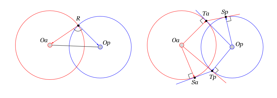
The figure shows the geometric interpretation of the scalar product of circles (2-dimensional spheres). At the left - definition through the scalar product of adjacent pairs and . If the circles intersect, they have a common element. - an element of adjacency pairs.
The scalar product of spheres can be defined through their mutual degrees (shown in the figure to the right). The geometric definition of the degree of a point is given in the 2nd part. According to (2.9) the degree of a point relative to the sphere is expressed through the distance from the point to the sphere and the norm of the sphere :
We can generalize this definition if we use another sphere instead of a point. Then the mutual degree of the two spheres and is the next scalar :
This formula is known as the Darboux product . The right figure shows the construction of points belonging to spheres, the distance between which is equal to the mutual degree of the spheres:
According to its properties, the mutual degree of spheres generalizes the properties of the degree of a point, that is, determines the relative position of the spheres. If the spheres are outside each other, then their mutual degree is positive; if they intersect, they are negative. By intersection here is meant the situation in which the touch points (or ) are inside the sphere (or respectively) (in the figure, the mutual degree of the spheres is positive).
Then the scalar product (5.5) is a mutual semi-degree of spheres (and vice versa). Recall (2.10) that by degree is understood the degree divided by (-2):
If the vertices of the spheres coincide ( ), their scalar product will be equal to the average norm of the spheres:
If the bases belong to different spaces, then the geometric interpretation of their scalar product complicated. First we give algebraic identities. They are similar to those for the components of the Laplace tensor given in the first part .
The scalar product of bases can be expressed in terms of the ratio of the determinants of the distance transition matrix and its main minor (see 5.1.1):
The relationship between the mutual norm of the bases and the barycentric coordinates of the back projections of their centers of spheres:
- for base vertices .
- for base vertices .
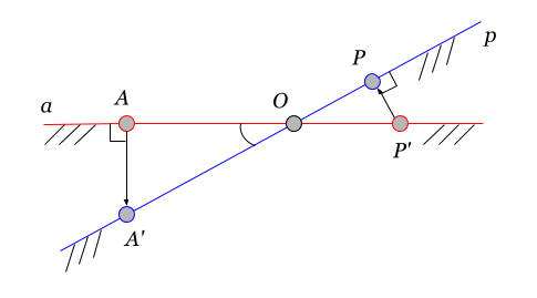
Let us see what a back projection of a point is. Suppose we have a point belonging to the base . Then its reverse projection on the basis there will be such a point that perpendicular dropped from it to the base intersects with it at the starting point .
In the figure, the reverse projection of a point on space is the point , and inverse projection point on space - point . Points and - these are centers of the sphere of bases. and respectively.
The concept of rear projection also applies to the norms of the spheres. The norm at the back projection becomes larger than the initial one (in contrast to the direct projection). In the figure, the distance - this is the norm of the basis sphere . Back projection on the basis there will be a distance:
.
Accordingly, the reverse projection of the norm basis on the basis of there will be a distance
.
Denoting the distance between reverse projections of centers as , we obtain the following expression for the scalar product of bases of different spaces:
We see that in form it coincides with the mutual norm of bases of one space (5.5), but instead of distances, their back projections onto a mutual basis are used. If the bases belong to the same space, then the angle between the spaces becomes zero, and formula (5.9) goes into (5.5).
All the above formulas are also applicable to the space of the graph. There are no spheres (basis) described in the graph, but there is a connection. Then the scalar product of graph bases should reflect their interconnection. But the question of the interpretation of this scalar (mutual norm of subgraphs) requires research.
Here we also consider two situations: 1) the new and the old basis belong to the same space and 2) belong to different spaces. The first case, as a rule, refers to the usual geometric space (when the basis is changed, its space rarely changes), the second to the space of the graph.
It is possible to determine the belonging of an element (vertex) to a basis space by its norm in the given space. If it is zero, then the element belongs to space.
To get the Gramian a new basis it is necessary to multiply the di-coordinates of the elements of the new basis on bi-coordinates . The resulting matrix will be the matrix of scalar products in the new basis (see 4.4.2 in the previous part ). Thus, if the spaces of the bases coincide, then the matrix of the norms of the vertices of the new basis with respect to the old is the grammian of the new basis:
We marked this Gramian with a stroke to remember the condition of a common space of bases. The Laplacian of the new basis (LMT) can be obtained by inversion of the Gramian (DMT):
The coordinates of the element in the new basis can be expressed in terms of the coordinates in the old and the transition matrix. Di-coordinates :
Element bi-coordinates in a new basis :
All the above expressions are similar to the formulas for changing coordinates in ordinary (vector) coordinate systems. Within a common space, the use of a point basis is similar to the use of a vector.
If the bases are in different spaces, then the formula (5.10.1) will give incorrect values of the half-distances between the vertices of the new basis. In the previous part it was shown that in the general case, to find the correct distances between the vertices, it is necessary to add the fundamental matrix to the norm matrix. (4.5):
Therefore, when transforming a basis to a basis from another space, it is necessary, along with the transition matrices, to specify the fundamental matrix of the new basis (relative to the original).
To define a fundamental matrix, it is useful to recall its geometric meaning (see 4.6.1 ). The element of the fundamental matrix is the scalar product of normals directed to the vertices of their projections onto the basis space. In the particular (but practically important) case of a common superspace, the element of the fundamental matrix is calculated as the product of the distances from the given elements to the basis space.
In the space of the graph, the values of the fundamental matrix can be obtained through the adjacency matrix between the old and the new basis . The elements of this matrix is the weight of the connections between the vertices of the two bases. If the matrix is known and reversible, then we can obtain the inverse adjacency matrix:
The resulting matrix (as well as the adjacency matrix) is an invariant — its values do not depend on the choice of the basis. Matrix element values reflect the scalar product of the back projections between the vertices of two bases. The figure shows an explanatory diagram.
Here point A belongs to the basis and point P is basis . The strokes mark the back projections of points on the adjacent basis. Then the value of the matrix element is the scalar product of vectors. and :
This ratio can be expressed in terms of the distances from the vertices to the hyperplane of intersection of the spaces (in the figure is the point O ) and the angle between the spaces :
From the formula (5.13.2 ') it is clear that if the bases are orthogonal , then the elements of the inner product turn to infinity.
It is convenient to give the dimension of the matrix of scalar products of projections to the dimension of the remaining transition matrices, edging it with zeros. Then the fundamental basis matrix defined as
Combining everything together, we get the final expression for the grammian of the new basis :
The source basis is expressed in a symmetric way with given transformation matrices:
Here and - bi-coordinates of transition matrices (5.2.1) and (5.2.2). - common remote transformation matrix:
This matrix is an invariant, consists of two parts - the remote transformation tensor and additives associated with the non-coplanarity of the basis spaces - the matrix of scalar products of projections .
The Laplace tensor of bases is obtained by inverting DMT (5.15). The problem of determining the connection of bases is solved.
Summing up. The heavy formula part of the series as a whole is complete. The basic concepts and identities are given. Point bases are a useful and powerful tool for various application tasks. In the final article we consider the basis of the simplest structure - in the form of a star.
Table of contents
In the previous part , the definition of a low dimension basis in a high dimension space was considered and it was shown how to determine distances between vertices that do not belong to a space of a basis. When replacing the basis of the requirement of preserving the metric properties of the coordinate system is also key.
Basic Matrices
The transformation matrices (transition matrices) are usually understood as such matrices, when multiplied by the coordinates of the element (vertex) in the old basis, its coordinates are obtained in the new one. Based on these matrices, metric tensors are also converted from one basis to another.
The basis transformation matrices contain the comparative characteristics of the two bases. Among these matrices, invariant matrices stand out — their values do not depend on the choice of the basis. For example, the matrix of distances between vertices is invariant.
')
Straight transition matrices
The set of initial base vertices is denoted as (old basis), new set as (new basis). For the coordinate transformation, the transition matrix must be specified - the description of the coordinates of the vertices of the new base in the old one. Such coordinates can be both di-coordinates of vertices and bi-coordinates. The transition matrix in di-coordinates is denoted as . The row of the matrix is the coordinates of the vertex of the new basis in the old respectively, the column is the di-coordinates of the vertex of the old basis relative to the new.
The transition matrix must be square, therefore the vertex coordinates alone are not enough - their number is less than the number of coordinate components (due to the presence of a scalar component in the coordinates). Therefore, it is necessary to add the di-coordinates of the normal vector [0; 1, 1, ... 1]. After that, the transition matrix in di-coordinates becomes similar in shape to the major Gramian. Let's call the matrix remote coordinate transformation tensor (DTP):
The distance transform tensor is an invariant — its values do not depend on the basis. On the reverse transition (from to ) the values of this matrix are simply transposed (rows and columns are swapped).
Since road accidents are di-coordinates, then multiplying them by the Laplacian (LMT), you can get the bi-coordinates . The structure of the bi-coordinates of the transition matrix:
The first row of this matrix is the b-coordinates of the normal: .
Unlike road accidents, the values of the bi-coordinates of the transition matrix depend on which basis they are obtained for — the old or the new. The choice of basis determines the matrix LMT. For definiteness, the bi-coordinate of the transition in the basis denote as , and in basis as . Then the following identities hold. For baseline:
,
and for new:
,
Here and - Laplacian and Gramian of the original basis. Respectively and - metric tensors of a new basis.
When moving from one basis to another, it is necessary to define the metric tensors of a new basis if the transformation matrices are specified.
Inverse transition matrices
Transition matrices and reversible subject to a non-zero determinant of the transition matrix:
or
The zero determinant of the transformation matrix means the orthogonality of the bases. In the orthogonal basis, it is impossible to express the metric of projections. We will consider bases non-orthogonal. Then the inverse transition matrices are expressed through the direct as follows:
Matrix - represents the bi-coordinates of the vertices of the old base with respect to the vertices of the new . That is, the inversion of bi-coordinates gives mutual bi-coordinates.
Matrix - this is the Laplace baseline transformation tensor (LTP). Its structure is similar to the structure of the Laplacian (LMT):
Here the major minor - This is a symmetric Laplacian. In the bordering are the barycentric coordinates of the reverse projections of the spheres of two bases (simplexes). The sphere of the original basis is expressed in the barycentric coordinates of the new - , and the sphere of the new in the coordinates of the original - .
What is meant by “reverse projections” will be explained further.
In the corner of the Laplace tensor is a scalar . Its value reflects the scalar product of two bases, the new and the old. To reveal its meaning, we consider two situations - 1) bases belong to the same space and 2) bases belong to different spaces.
Scalar product of bases of one space
In the common space, the scalar product of bases is expressed in terms of the norms of basic spheres ( and ) and the distance between the centers of the spheres ( ):
This formula is similar to the expression for the scalar product of pairs with a common vertex (3.8) . Therefore, we can consider relation (5.5) to be the definition of the scalar product of hyperspheres or simplices belonging to the same space.
The figure shows the geometric interpretation of the scalar product of circles (2-dimensional spheres). At the left - definition through the scalar product of adjacent pairs and . If the circles intersect, they have a common element. - an element of adjacency pairs.
The scalar product of spheres can be defined through their mutual degrees (shown in the figure to the right). The geometric definition of the degree of a point is given in the 2nd part. According to (2.9) the degree of a point relative to the sphere is expressed through the distance from the point to the sphere and the norm of the sphere :
We can generalize this definition if we use another sphere instead of a point. Then the mutual degree of the two spheres and is the next scalar :
This formula is known as the Darboux product . The right figure shows the construction of points belonging to spheres, the distance between which is equal to the mutual degree of the spheres:
According to its properties, the mutual degree of spheres generalizes the properties of the degree of a point, that is, determines the relative position of the spheres. If the spheres are outside each other, then their mutual degree is positive; if they intersect, they are negative. By intersection here is meant the situation in which the touch points (or ) are inside the sphere (or respectively) (in the figure, the mutual degree of the spheres is positive).
Then the scalar product (5.5) is a mutual semi-degree of spheres (and vice versa). Recall (2.10) that by degree is understood the degree divided by (-2):
If the vertices of the spheres coincide ( ), their scalar product will be equal to the average norm of the spheres:
Scalar product of bases of different spaces
If the bases belong to different spaces, then the geometric interpretation of their scalar product complicated. First we give algebraic identities. They are similar to those for the components of the Laplace tensor given in the first part .
The scalar product of bases can be expressed in terms of the ratio of the determinants of the distance transition matrix and its main minor (see 5.1.1):
The relationship between the mutual norm of the bases and the barycentric coordinates of the back projections of their centers of spheres:
- for base vertices .
- for base vertices .
Let us see what a back projection of a point is. Suppose we have a point belonging to the base . Then its reverse projection on the basis there will be such a point that perpendicular dropped from it to the base intersects with it at the starting point .
In the figure, the reverse projection of a point on space is the point , and inverse projection point on space - point . Points and - these are centers of the sphere of bases. and respectively.
The concept of rear projection also applies to the norms of the spheres. The norm at the back projection becomes larger than the initial one (in contrast to the direct projection). In the figure, the distance - this is the norm of the basis sphere . Back projection on the basis there will be a distance:
.
Accordingly, the reverse projection of the norm basis on the basis of there will be a distance
.
Denoting the distance between reverse projections of centers as , we obtain the following expression for the scalar product of bases of different spaces:
We see that in form it coincides with the mutual norm of bases of one space (5.5), but instead of distances, their back projections onto a mutual basis are used. If the bases belong to the same space, then the angle between the spaces becomes zero, and formula (5.9) goes into (5.5).
All the above formulas are also applicable to the space of the graph. There are no spheres (basis) described in the graph, but there is a connection. Then the scalar product of graph bases should reflect their interconnection. But the question of the interpretation of this scalar (mutual norm of subgraphs) requires research.
Calculation of the new basis
Here we also consider two situations: 1) the new and the old basis belong to the same space and 2) belong to different spaces. The first case, as a rule, refers to the usual geometric space (when the basis is changed, its space rarely changes), the second to the space of the graph.
It is possible to determine the belonging of an element (vertex) to a basis space by its norm in the given space. If it is zero, then the element belongs to space.
Common space of bases
To get the Gramian a new basis it is necessary to multiply the di-coordinates of the elements of the new basis on bi-coordinates . The resulting matrix will be the matrix of scalar products in the new basis (see 4.4.2 in the previous part ). Thus, if the spaces of the bases coincide, then the matrix of the norms of the vertices of the new basis with respect to the old is the grammian of the new basis:
We marked this Gramian with a stroke to remember the condition of a common space of bases. The Laplacian of the new basis (LMT) can be obtained by inversion of the Gramian (DMT):
The coordinates of the element in the new basis can be expressed in terms of the coordinates in the old and the transition matrix. Di-coordinates :
Element bi-coordinates in a new basis :
All the above expressions are similar to the formulas for changing coordinates in ordinary (vector) coordinate systems. Within a common space, the use of a point basis is similar to the use of a vector.
Example of base conversion
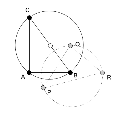
KDPV shows the main basis from 3 vertices ( A, B, C ) and a new basis formed by vertices ( P, Q, R ). The values of the DMT of the main basis are in the first article :
\ begin {array} {c | cccc}
Gm_ {aa} & * & A & B & C \\
\ hline
* & 0 & 1 & 1 & 1 \\
A & 1 & 0 & -4.5 & -8 \\
B & 1 & -4.5 & 0 & -12.5 \\
C & 1 & -8 & -12.5 & 0 \\
\ end {array}
An asterisk denotes a scalar component. The value of the Laplacian (LMT) can be obtained by inverting the Gramian (DMT).
The remote transition matrix is assumed to be given. Her appearance:
\ begin {array} {c | cccc}
Dm_ {pa} & * & A & B & C \\
\ hline
* & 0 & 1 & 1 & 1 \\
P & 1 & -1.0 & -2.5 & -13.0 \\
Q & 1 & -6.5 & -2.0 & -6.5 \\
R & 1 & -12.5 & -2.0 & -20.5 \\
\ end {array}
The values of the bi-coordinates of the transition matrix are obtained by the formula (5.2.1):
\ begin {array} {c | cccc}
Ba_p {} ^ a & * & A & B & C \\
\ hline
* & 1 & 0 & 0 & 0 \\
P & -1.5 & 0.91 (6) & 0. (3) & -0.25 \\
Q & 2.0 & -0.5 & 1.0 & 0.50 \\
R & -5.0 & -0. (6) & 1. (6) & 0.0 \\
\ end {array}
The scalar component (values of the first column) of the bi-coordinates are the orbitals. The sum of the barycentric components is 1.
Laplace transform tensor (5.3.1):
\ begin {array} {c | cccc}
Lt ^ {ap} & * & P & Q & R \\
\ hline
* & 2.15 & 0.30 & 1.15 & -0.45 \\
A & 0.058 (3) & 0.11 (6) & -0.0 (6) & -0.05 \\
B & 0.9 (6) & -0.0 (6) & -0.0 (3) & 0.10 \\
C & -0.025 & -0.05 & 0.10 & -0.05 \\
\ end {array}
Vector - these are the barycentric coordinates of the center of the sphere of the old basis ( ABC simplex) relative to the vertices of the new ( PQR ). Accordingly, the vector - conversely, the barycentric coordinates of the center of the described sphere of the PQR simplex with respect to the vertices of the old basis.
Using (5.10.1), we get the Gramian of a new basis:
\ begin {array} {c | cccc}
Gm '_ {pp} & * & P & Q & R \\
\ hline
* & 0 & 1 & 1 & 1 \\
P & 1 & 0 & -6.5 & -8.5 \\
Q & 1 & -6.5 & 0 & -4.0 \\
R & 1 & -8.5 & -4.0 & 0 \\
\ end {array}
\ begin {array} {c | cccc}
Gm_ {aa} & * & A & B & C \\
\ hline
* & 0 & 1 & 1 & 1 \\
A & 1 & 0 & -4.5 & -8 \\
B & 1 & -4.5 & 0 & -12.5 \\
C & 1 & -8 & -12.5 & 0 \\
\ end {array}
An asterisk denotes a scalar component. The value of the Laplacian (LMT) can be obtained by inverting the Gramian (DMT).
The remote transition matrix is assumed to be given. Her appearance:
\ begin {array} {c | cccc}
Dm_ {pa} & * & A & B & C \\
\ hline
* & 0 & 1 & 1 & 1 \\
P & 1 & -1.0 & -2.5 & -13.0 \\
Q & 1 & -6.5 & -2.0 & -6.5 \\
R & 1 & -12.5 & -2.0 & -20.5 \\
\ end {array}
The values of the bi-coordinates of the transition matrix are obtained by the formula (5.2.1):
\ begin {array} {c | cccc}
Ba_p {} ^ a & * & A & B & C \\
\ hline
* & 1 & 0 & 0 & 0 \\
P & -1.5 & 0.91 (6) & 0. (3) & -0.25 \\
Q & 2.0 & -0.5 & 1.0 & 0.50 \\
R & -5.0 & -0. (6) & 1. (6) & 0.0 \\
\ end {array}
The scalar component (values of the first column) of the bi-coordinates are the orbitals. The sum of the barycentric components is 1.
Laplace transform tensor (5.3.1):
\ begin {array} {c | cccc}
Lt ^ {ap} & * & P & Q & R \\
\ hline
* & 2.15 & 0.30 & 1.15 & -0.45 \\
A & 0.058 (3) & 0.11 (6) & -0.0 (6) & -0.05 \\
B & 0.9 (6) & -0.0 (6) & -0.0 (3) & 0.10 \\
C & -0.025 & -0.05 & 0.10 & -0.05 \\
\ end {array}
Vector - these are the barycentric coordinates of the center of the sphere of the old basis ( ABC simplex) relative to the vertices of the new ( PQR ). Accordingly, the vector - conversely, the barycentric coordinates of the center of the described sphere of the PQR simplex with respect to the vertices of the old basis.
Using (5.10.1), we get the Gramian of a new basis:
\ begin {array} {c | cccc}
Gm '_ {pp} & * & P & Q & R \\
\ hline
* & 0 & 1 & 1 & 1 \\
P & 1 & 0 & -6.5 & -8.5 \\
Q & 1 & -6.5 & 0 & -4.0 \\
R & 1 & -8.5 & -4.0 & 0 \\
\ end {array}
Bases in different spaces
If the bases are in different spaces, then the formula (5.10.1) will give incorrect values of the half-distances between the vertices of the new basis. In the previous part it was shown that in the general case, to find the correct distances between the vertices, it is necessary to add the fundamental matrix to the norm matrix. (4.5):
Therefore, when transforming a basis to a basis from another space, it is necessary, along with the transition matrices, to specify the fundamental matrix of the new basis (relative to the original).
To define a fundamental matrix, it is useful to recall its geometric meaning (see 4.6.1 ). The element of the fundamental matrix is the scalar product of normals directed to the vertices of their projections onto the basis space. In the particular (but practically important) case of a common superspace, the element of the fundamental matrix is calculated as the product of the distances from the given elements to the basis space.
Scalar product of back projections
In the space of the graph, the values of the fundamental matrix can be obtained through the adjacency matrix between the old and the new basis . The elements of this matrix is the weight of the connections between the vertices of the two bases. If the matrix is known and reversible, then we can obtain the inverse adjacency matrix:
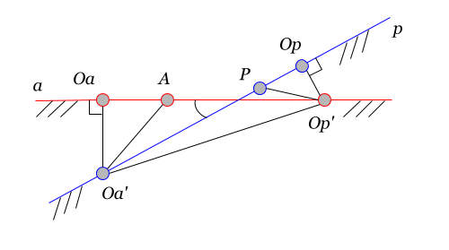
The resulting matrix (as well as the adjacency matrix) is an invariant — its values do not depend on the choice of the basis. Matrix element values reflect the scalar product of the back projections between the vertices of two bases. The figure shows an explanatory diagram.
Here point A belongs to the basis and point P is basis . The strokes mark the back projections of points on the adjacent basis. Then the value of the matrix element is the scalar product of vectors. and :
This ratio can be expressed in terms of the distances from the vertices to the hyperplane of intersection of the spaces (in the figure is the point O ) and the angle between the spaces :
From the formula (5.13.2 ') it is clear that if the bases are orthogonal , then the elements of the inner product turn to infinity.
Total basis conversion formulas
It is convenient to give the dimension of the matrix of scalar products of projections to the dimension of the remaining transition matrices, edging it with zeros. Then the fundamental basis matrix defined as
Combining everything together, we get the final expression for the grammian of the new basis :
The source basis is expressed in a symmetric way with given transformation matrices:
Here and - bi-coordinates of transition matrices (5.2.1) and (5.2.2). - common remote transformation matrix:
This matrix is an invariant, consists of two parts - the remote transformation tensor and additives associated with the non-coplanarity of the basis spaces - the matrix of scalar products of projections .
The Laplace tensor of bases is obtained by inverting DMT (5.15). The problem of determining the connection of bases is solved.
Summing up. The heavy formula part of the series as a whole is complete. The basic concepts and identities are given. Point bases are a useful and powerful tool for various application tasks. In the final article we consider the basis of the simplest structure - in the form of a star.
Source: https://habr.com/ru/post/339968/
All Articles