Development for Sailfish OS: displaying graphs using D3.js and QML Canvas
Hello! This article is a continuation of a series of articles devoted to the development of applications for the Sailfish OS mobile platform. This time it will be about working with graphs in the Sailfish application. We will talk about the search and connection of the library and how we display graphs of mathematical functions. Note that the proposed solution is not limited to the Saiflsh OS platform and is generally suitable for any QtQuick application.
We decided to create a calculator application that would satisfy the needs of engineers, students and schoolchildren working with devices running Sailfish OS. Our application should contain the following components:
We decided to add graph display functionality to the equation solution block. To solve this problem within the framework of a QML application, the following approaches can be applied:
The QuickQanava library works with Qt 5.8, which is not yet available on the Sailfish OS platform. The QML Canvas object allows you to use a high-level JavaScript language, and also provides an API that is compatible with the W3C standard, which opens up possibilities for using third-party libraries.
')
Due to the fact that the display of the graphics does not require serious calculations and we do not need to redraw the scene often, we decided to use the QML Canvas in the project with the help of an external JavaScript library.
The QML Canvas element allows you to draw straight and curved lines, simple and complex shapes, graphics, and links to graphic images. It can also draw text, colors, shadows, gradients and patterns, as well as perform image manipulation at the pixel level. In addition to displaying the Canvas output, the output can be saved as an image file or serialized into a URL.
Rendering to canvas is done using a Context2D object, usually as a result of the paint signal processing. The object itself implements the HTML Canvas 2D Context specification, which is also implemented in the HTML Canvas object, which allows the use of JavaScript libraries designed for use in web browsers for QML applications. Currently, three-dimensional context is not supported by the Context2D object.
Consider the simplest example of connecting a QML Canvas to your application:
The first line in the example is to connect QtQuick 2.0 , then define the Canvas element and set the parameters id , width and height . Since the element itself has no elements and can occupy arbitrary space, it is necessary for it to specify the dimensions either by explicitly specifying the width and height, or by associating the edges of the element with other elements on the page. If you do not specify a size, the item will not be visible. In the example we use the first approach.
The paint signal is called when the Canvas element is activated. Its processing takes place in the onPaint method. In it, we get the context to display and store it in the variable ctx . A full description of the parameters for getContext can be, for example, here . Be careful, Qt only provides access to a two-dimensional display context.
Next we use the context to display the rectangle. ctx.fillStyle sets the fill color of the rectangle. The first three parameters determine the color of the components red, green and blue, and the fourth component determines the transparency. ctx.fillRect (x, y, w, h) draws it using x and y as the coordinates of the beginning, and w and h as the width and height.
The entire list of context methods that can be used for drawing can be found in the official documentation . We will not consider all the methods in this article, we only note that the coordinates of the image begin in the upper left corner. The OX axis is growing to the right, and the OY axis is from top to bottom.
Of course, we could solve the problem we were given directly using the Context2D API, however we decided to consider the possibility of using external libraries. Due to the fact that this API is available in all major browsers, developers under Sailfish OS can use a large number of existing libraries that facilitate the implementation of target functions. In our application, we decided to use the D3.js library .
D3.js is a JavaScript library for processing and visualizing data. Currently D3.js is one of the most popular frameworks used for graphical data processing and creating all kinds of charts and graphs.
D3.js itself is a large project that allows you to solve many problems, so there is no single way to integrate this library into HTML applications. We used a fairly simple approach for integration, but others should also work successfully in your applications.
First you need to download the library and make it available on the target device. We remind you that QML components on Sailfish OS are not compiled into resources, but are delivered as separate files. As a result, all dependencies on JavaScript are also desirable to deliver as separate files.
D3.js comes in a separate file called d3.js, as well as a minified version that is in the d3.min.js file. During development, we found out that the minified version does not load correctly with the QML engine, so it is recommended to use the full version - it works without complaints.
For our application, we placed the d3.js file in the qml / pages directory of our project. The entire contents of this directory is copied to the target device, so the file is also copied with the project. The file was also included in the DISTFILES list in the QML project, so that QtCreator would show it in the list of other files.
Within the framework of the application, we need to display graphs of three functions on a two-dimensional plane. All considered functions depend on the value of the abscissa. For the qualitative display of them on the segment, we decided to calculate the intermediate values on the currently displayed segment.
We constructed the general logic by construction in a separate component Plot . It provides the following functionality:
In specific places of use, we need to define only 1 function that will calculate the values of the graph.
Consider the structure of the base component.
First, we include the libraries we need: the QtQuick component set, as well as the D3.js library itself. Connecting JavaScript files is similar to connecting other QML files. To solve this problem, the import keyword is also used.
Full information about connecting JavaScript files can be found in the official documentation . The main aspect of the import process is the indication of the name through which all the functions defined in this document will be available. In our code, we have named this object D3 .
The root element of the Plot is Canvas , on which we display information. To perform calculations and gesture processing in this element, we defined a set of properties and functions. The key one is onPaint - an event handler for image rendering.
The child element in relation to Canvas is Item , which is just a container for PinchArea and MouseArea objects . These objects were added to process a pinch, to control the level of approximation, and to drag, to control the position of the coordinate axes. Gesture data handlers update coordinates that are used when drawing graphics.
We will not consider the process of drawing step by step, since it does not represent much interest on the one hand, and on the other hand you can look at the source code of the application and understand the details yourself. At the same time, we will look at important points that may cause difficulties.
To display the key elements: the coordinate grid and the graph of the function, the d3.line function is used. This function allows you to display arbitrary polylines and straight lines. The input to the function is an array of data. In order to use it, you must configure the following parameters:
Consider an example of the formation of the image line graph.
First, we adjust the scales, d3.scaleLinear , which simplify our work with scaling the graph. It suffices to specify the physical boundaries of the image in the call to the range () method and the boundaries of the graph in the call to the domain () method. The scales for the abscissa and ordinates are formed and are recorded in the variables xScale and yScale , respectively.
Then we describe a line that will take an array of graph values as parameters. In the x () method call, we pass a function that extracts the first element of the array and converts it using the xScale scale. A similar function is passed as an argument to the method call y () , only the call is made to the second element of the array. Then we set up the way of communication between the elements, in our case it is d3.curveNatural . D3.js supports a huge number of options for constructing curves, you can read about them in the official documentation . At the end of the line we connect it with the graphic context of our image.
To draw a line, it is enough to call the created line and pass an array of necessary coordinates to it:
Similarly, lines are drawn to display axes.
It should be noted that at the beginning of each drawing the canvas is completely cleared. This is necessary so that the previous image does not interfere with the display of the current state. And new images appear when the user changes the scale of the graph or changes the borders of the display elements.
With this component, we implemented the display of three graphs for each of the functions. For each graphic we created a page by page. On these pages, the values are calculated to display the graph.
The overall structure of each graph is shown below.
The root element is the page that is placed on the stack to display the graph. The parameters are the coefficients of the equation, the initial boundaries for the display of the graph, as well as the line showing the location of the roots of the function.
Next, we disable navigation back if the user interacts with the schedule. This helps prevent accidental returns from the page using gestures.
The only element on the page is the Plot element. We explicitly indicate that it takes up all the available space, it will be used to display the graph. We also define the drawPlot method. This method will be called each time you need to re-display the function.
As an argument, it is passed a line that was configured, as shown above, in the Plot element. We call it and pass it the result of the getPoints () method. The latter method forms a set of points that will be specific to each individual graph.
We hope that using this information you can easily implement this functionality in your application. You can also learn more about the implementation of functions in the Matrix Calculator application by installing it from the OpenRepos.net repository, or look at working with the library in source code that is available in the repository on BitBucket .
Screenshots of the application are shown below:
UPD : Added screenshots of the application.
Task Description
We decided to create a calculator application that would satisfy the needs of engineers, students and schoolchildren working with devices running Sailfish OS. Our application should contain the following components:
- Calculator with two modes of operation: simple and advanced.
- A subsystem of matrix calculations that supports addition, multiplication of matrices, calculation of their rank and determinant, as well as transposition.
- The block solving the following equations: power equations up to 4 degrees, exponential and trigonometric equations.
We decided to add graph display functionality to the equation solution block. To solve this problem within the framework of a QML application, the following approaches can be applied:
- Connect an external library like QuickQanava .
- Use a QML Canvas object.
- Implement your own component in C ++ and connect it to the application.
The QuickQanava library works with Qt 5.8, which is not yet available on the Sailfish OS platform. The QML Canvas object allows you to use a high-level JavaScript language, and also provides an API that is compatible with the W3C standard, which opens up possibilities for using third-party libraries.
')
Due to the fact that the display of the graphics does not require serious calculations and we do not need to redraw the scene often, we decided to use the QML Canvas in the project with the help of an external JavaScript library.
QML Canvas and Context2D
The QML Canvas element allows you to draw straight and curved lines, simple and complex shapes, graphics, and links to graphic images. It can also draw text, colors, shadows, gradients and patterns, as well as perform image manipulation at the pixel level. In addition to displaying the Canvas output, the output can be saved as an image file or serialized into a URL.
Rendering to canvas is done using a Context2D object, usually as a result of the paint signal processing. The object itself implements the HTML Canvas 2D Context specification, which is also implemented in the HTML Canvas object, which allows the use of JavaScript libraries designed for use in web browsers for QML applications. Currently, three-dimensional context is not supported by the Context2D object.
Consider the simplest example of connecting a QML Canvas to your application:
import QtQuick 2.0 Canvas { id: mycanvas width: 100 height: 200 onPaint: { var ctx = getContext("2d"); ctx.fillStyle = Qt.rgba(1, 0, 0, 1); ctx.fillRect(0, 0, width, height); } } The first line in the example is to connect QtQuick 2.0 , then define the Canvas element and set the parameters id , width and height . Since the element itself has no elements and can occupy arbitrary space, it is necessary for it to specify the dimensions either by explicitly specifying the width and height, or by associating the edges of the element with other elements on the page. If you do not specify a size, the item will not be visible. In the example we use the first approach.
The paint signal is called when the Canvas element is activated. Its processing takes place in the onPaint method. In it, we get the context to display and store it in the variable ctx . A full description of the parameters for getContext can be, for example, here . Be careful, Qt only provides access to a two-dimensional display context.
Next we use the context to display the rectangle. ctx.fillStyle sets the fill color of the rectangle. The first three parameters determine the color of the components red, green and blue, and the fourth component determines the transparency. ctx.fillRect (x, y, w, h) draws it using x and y as the coordinates of the beginning, and w and h as the width and height.
The entire list of context methods that can be used for drawing can be found in the official documentation . We will not consider all the methods in this article, we only note that the coordinates of the image begin in the upper left corner. The OX axis is growing to the right, and the OY axis is from top to bottom.
Using external libraries
Of course, we could solve the problem we were given directly using the Context2D API, however we decided to consider the possibility of using external libraries. Due to the fact that this API is available in all major browsers, developers under Sailfish OS can use a large number of existing libraries that facilitate the implementation of target functions. In our application, we decided to use the D3.js library .
D3.js Short Review
D3.js is a JavaScript library for processing and visualizing data. Currently D3.js is one of the most popular frameworks used for graphical data processing and creating all kinds of charts and graphs.
D3.js itself is a large project that allows you to solve many problems, so there is no single way to integrate this library into HTML applications. We used a fairly simple approach for integration, but others should also work successfully in your applications.
Integrating D3.js into a QML application
First you need to download the library and make it available on the target device. We remind you that QML components on Sailfish OS are not compiled into resources, but are delivered as separate files. As a result, all dependencies on JavaScript are also desirable to deliver as separate files.
D3.js comes in a separate file called d3.js, as well as a minified version that is in the d3.min.js file. During development, we found out that the minified version does not load correctly with the QML engine, so it is recommended to use the full version - it works without complaints.
For our application, we placed the d3.js file in the qml / pages directory of our project. The entire contents of this directory is copied to the target device, so the file is also copied with the project. The file was also included in the DISTFILES list in the QML project, so that QtCreator would show it in the list of other files.
Creating a component to display the graph
Within the framework of the application, we need to display graphs of three functions on a two-dimensional plane. All considered functions depend on the value of the abscissa. For the qualitative display of them on the segment, we decided to calculate the intermediate values on the currently displayed segment.
We constructed the general logic by construction in a separate component Plot . It provides the following functionality:
- Displays the grid with captions.
- Change the displayed coordinates using gestures.
- Graph display based on calculated values. The specific function must be implemented at the point of use, the base type does not provide this function.
In specific places of use, we need to define only 1 function that will calculate the values of the graph.
Consider the structure of the base component.
import QtQuick 2.0 import "d3.js" as D3 Canvas { // onPaint { } // // Item { PinchArea {} // MouseArea {} // } } First, we include the libraries we need: the QtQuick component set, as well as the D3.js library itself. Connecting JavaScript files is similar to connecting other QML files. To solve this problem, the import keyword is also used.
Full information about connecting JavaScript files can be found in the official documentation . The main aspect of the import process is the indication of the name through which all the functions defined in this document will be available. In our code, we have named this object D3 .
The root element of the Plot is Canvas , on which we display information. To perform calculations and gesture processing in this element, we defined a set of properties and functions. The key one is onPaint - an event handler for image rendering.
The child element in relation to Canvas is Item , which is just a container for PinchArea and MouseArea objects . These objects were added to process a pinch, to control the level of approximation, and to drag, to control the position of the coordinate axes. Gesture data handlers update coordinates that are used when drawing graphics.
Overview of the mapping process
We will not consider the process of drawing step by step, since it does not represent much interest on the one hand, and on the other hand you can look at the source code of the application and understand the details yourself. At the same time, we will look at important points that may cause difficulties.
To display the key elements: the coordinate grid and the graph of the function, the d3.line function is used. This function allows you to display arbitrary polylines and straight lines. The input to the function is an array of data. In order to use it, you must configure the following parameters:
- Configure the generators to obtain ordinates and abscissas from the array element.
- Specify the method of connecting the lines together.
- Specify the graphic context in which to display the information.
Consider an example of the formation of the image line graph.
var context = plot.getContext('2d'); var xScale = d3.scaleLinear() .range([leftMargin, width]) .domain([minX, maxX]); var yScale = d3.scaleLinear() .range([height - bottomMargin, 0]) .domain([minY, maxY]); var line = d3.line().x(function (d) { return xScale(d[0]); }).y(function (d) { return yScale(d[1]); }).curve(d3.curveNatural).context(context); First, we adjust the scales, d3.scaleLinear , which simplify our work with scaling the graph. It suffices to specify the physical boundaries of the image in the call to the range () method and the boundaries of the graph in the call to the domain () method. The scales for the abscissa and ordinates are formed and are recorded in the variables xScale and yScale , respectively.
Then we describe a line that will take an array of graph values as parameters. In the x () method call, we pass a function that extracts the first element of the array and converts it using the xScale scale. A similar function is passed as an argument to the method call y () , only the call is made to the second element of the array. Then we set up the way of communication between the elements, in our case it is d3.curveNatural . D3.js supports a huge number of options for constructing curves, you can read about them in the official documentation . At the end of the line we connect it with the graphic context of our image.
To draw a line, it is enough to call the created line and pass an array of necessary coordinates to it:
line([[1, 2], [2, 15], [3, 8], [4, 6]]) Similarly, lines are drawn to display axes.
It should be noted that at the beginning of each drawing the canvas is completely cleared. This is necessary so that the previous image does not interfere with the display of the current state. And new images appear when the user changes the scale of the graph or changes the borders of the display elements.
Using the Plot component
With this component, we implemented the display of three graphs for each of the functions. For each graphic we created a page by page. On these pages, the values are calculated to display the graph.
The overall structure of each graph is shown below.
Page { property var elem property var border property var rootLine id: page backNavigation: plot.controlNavigation() Plot { id: plot anchors.margins: Theme.horizontalPageMargin width: parent.width height: parent.height function drawPlot(line) { line(getPoints()); } function getPoints() { // . } } } The root element is the page that is placed on the stack to display the graph. The parameters are the coefficients of the equation, the initial boundaries for the display of the graph, as well as the line showing the location of the roots of the function.
Next, we disable navigation back if the user interacts with the schedule. This helps prevent accidental returns from the page using gestures.
The only element on the page is the Plot element. We explicitly indicate that it takes up all the available space, it will be used to display the graph. We also define the drawPlot method. This method will be called each time you need to re-display the function.
As an argument, it is passed a line that was configured, as shown above, in the Plot element. We call it and pass it the result of the getPoints () method. The latter method forms a set of points that will be specific to each individual graph.
Matrix Calculator application
We hope that using this information you can easily implement this functionality in your application. You can also learn more about the implementation of functions in the Matrix Calculator application by installing it from the OpenRepos.net repository, or look at working with the library in source code that is available in the repository on BitBucket .
Screenshots of the application are shown below:
 | 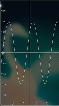 |
UPD : Added screenshots of the application.
Source: https://habr.com/ru/post/339930/
All Articles