How to determine the sample size?

Statistics knows everything. And Ilf and E. Petrov, "12 Chairs"

Imagine that you are building a large shopping center and you want to assess the traffic flow entering the parking area. No, let's give another example ... they will never do it anyway. You need to evaluate the taste preferences of visitors to your portal, for which you need to conduct a survey among them. How to reconcile the amount of data and the possible error? Nothing complicated - the larger your sample, the smaller the error. However, there are nuances.

Theoretical minimum

It would not be superfluous to refresh the memory, these terms will be useful to us further.

• Population - The set of all objects among which research is being conducted.
• Sample - A subset, part of the objects from the entire population that is directly involved in the study.
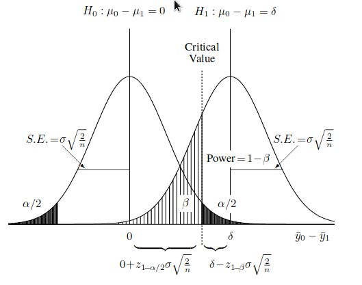
• Error of the first kind - (α) The probability of rejecting the null hypothesis, while it is true.
• Error of the second kind - (β) Probability not to reject the null hypothesis, while it is false.
• 1 - β - Statistical power of the criterion.
• μ ₀ and μ ₁ - Average values ​​for the null and alternative hypothesis.

Already in the very definitions of the errors of the first and second kind there is room for debate and interpretation. How to determine them and what to choose as zero? If you are investigating the level of contamination of soil or water, how do you formulate the null hypothesis: is there pollution or is there no pollution? But the size of the sample from the general population of objects depends on it.

The initial population , as well as the sample, can have any distribution, however the average value is normal or Gaussian distribution due to the Central Limit Theorem .

Regarding the distribution parameters and the average value in particular, several types of conclusions are possible. The first one is called the confidence interval . It indicates the interval of possible values ​​of the parameter, with the specified confidence factor . So for example, a 100(1-α)% confidence interval for μ would be (Lev. 1).

$$

$$\ hat {\ mu} \ pm t _ {{\ alpha / 2}; df} \ sqrt {\ frac {\ hat \ sigma ^ 2} {n}}$$

• df - the degree of freedom = n - 1, from the English "degrees of freedom".
• $$$t _ {{\ alpha / 2}; df}$- Two-sided critical value, t- .

The second conclusion is to test the hypothesis . It may be something like this.

• H ₀ : μ = h
• H ₁ : μ> h
• H ₂ : μ <h

With a confidence interval of 100(1-α) for μ, you can make a choice in favor of H ₁ and H ₂ :

• If the lower limit of the confidence interval is 100(1-α) < h , then we reject H ₀ in favor of H ₂ .
• If the upper limit of the confidence interval is 100(1-α) > h, then we reject H ₀ in favor of H ₁ .
• If the confidence interval of 100(1-α) includes h, then we cannot reject H ₀ and this result is considered undefined .

If we need to check the value of μ for one sample from the total population, then the criterion will take the form.

• Reject H ₀ and accept H ₁ : μ> h if $$$t> t _ {{\ alpha / 2}; df}$.
• Reject H ₀ and take H ₂ : μ <h if $$$t <t _ {{\ alpha / 2}; df}$.
• It is impossible to reject H ₀ if $$$| t | <t _ {{\ alpha / 2}; df}$.

Where $$$t = (\ hat {\ mu} - h) / \ sqrt \ frac {\ hat \ sigma ^ 2} {n}$.

Confidence interval, inaccuracy and sample size

Take the very first equation and express from there the width of the confidence interval (Lev. 2).

$$

$$w = 2t _ {{\ alpha / 2}; df} \ sqrt {\ frac {\ hat \ sigma ^ 2} {n}}$$

In some cases, we can replace the t- with z . With another simplification, we replace the half of w with the measurement error E. Then our equations take the form (Lev. 3).

$$

$$E = z _ {\ alpha / 2} \ sqrt {\ frac {\ hat \ sigma ^ 2} {n}}$$

As you can see, the error really decreases with increasing amount of input data . Whence it is easy to derive what is required (Lv. 4).

$$

$$n = \ left [\ frac {z _ {\ alpha / 2} * \ sigma} {E} \ right] ^ 2$$

Practice - count with R

Let us test the hypothesis that the average value of a given sample of the number of insects in a trap is 1.

• H ₀ : μ = 1
• H ₁ : μ> 1

Insects	0	one	2	3	four	five	6
Traps	ten	9	five	five	one	2	one

 > x <- read.table("/tmp/tcounts.txt") > y = unlist(x, use.names="false") > mean(z);sd(z) [1] 1.636364 [1] 1.654883 

Note that the mean and standard deviation are almost equal, which is natural for the Poisson distribution. The 95% confidence interval for t- and df=32 .

 > qt(.975, 32) [1] 2.036933 

and finally we get the critical interval for the average value: 1.05 - 2.22 .

 > μ=mean(z) > st = qt(.975, 32) > μ + st * sd(z)/sqrt(33) [1] 2.223159 > μ - st * sd(z)/sqrt(33) [1] 1.049568 

As a result, it is necessary to reject H ₀ and take H ₁ since with a probability of 95%, μ > 1.

In the same example, if we accept that we know the actual standard deviation - σ , and not its estimate obtained using a random sample, we can calculate the necessary n for a given error. Calculate for E=0.5 .

 > za2 = qnorm(.975) > (za2*sd(z)/.5)^2 [1] 42.08144 

Wind correction

In fact, there is no reason to believe that σ (variance) will be known to us, while we have yet to evaluate μ (mean). Because of this, equation 4 is of little practical use, except for particularly refined examples from the field of combinatorics, and a realistic equation for n somewhat more complicated with an unknown σ (Level 5).

$$

$$n = 4 \ tilde \ sigma ^ 2 (z _ {\ alpha / 2} / w) ^ 2 + z ^ 2 _ {\ alpha / 2} / 2$$

Note that σ in the last equation is not with a cap (^), but a tilde (~). This is due to the fact that at the very beginning we don’t even have an estimated standard deviation of a random sample - $$$\ hat \ sigma$, and instead we use the planned - $$$\ tilde \ sigma$. Where do we get the last? We can say that from the ceiling: expert assessment, rough estimates, past experience, etc.

And what about the second term of the right side of the 5th equation, where did it come from? Because $$$z _ {\ alpha / 2} <t _ {{\ alpha / 2}; df}$Gunther's amendment is needed.

In addition to equations 4 and 5, there are a few approximate formulas, but this already deserves a separate post.

Used materials

1. Sample sizes
2. Hypothesis testing