Data geometry 4. Graph space
A feature of coordinate systems on a point basis ( di- and bi-coordinates ) is that they can be used both in ordinary geometric space and in the space of a graph.

The dimension of the space of a graph is determined by the number of its connected vertices (we will assume that all the vertices of the graph are connected — a one-component graph). The basis of space is defined as a subset of the vertices of the graph with known distances between them (the metric). A subset may include all the vertices of the graph, or only a part (subgraph). In the latter case, the basis dimension is less than the dimension of the general space of the graph.
It is necessary to understand what are the elements and vectors on the graph. A graph is a set of related elements (nodes). The nodes of the graph determine its set of potential basic elements, and the connections - the metric, the distance between the basic elements.
As a basis for determining the coordinate system on a graph, not all nodes of the graph can be selected, but only a part of it - the base subgraph. In this case, the total space of the graph can be divided into two subspaces - basic and outside basic (external).
')
The nodes that are included in the basis of the graph are called basic. All other space elements are set relative to its base nodes through the barycentric coordinates (weights of the base vertices).
In the general case, an element can either belong to the space of a basis, or lie outside its limits. Elements outside the base will be called external . Since the outer element has a nonzero distance to the base space, each outer element is a graph node that is not included in its basis. That is, the external elements are explicitly specified in the structure of the graph.
The elements belonging to the space of a basis do not appear in any way in the structure - virtual elements (except for the directly defined vertices of the basis). The rate of virtual elements is zero — it is simply the vector of potentials normalized to unity at the vertices of the basis. An example of a virtual basis space element is the center of the described sphere.
If the graph is an electrical circuit, then the element is the set of potentials at the nodes of the network. The Laplacian of an electrical circuit is a matrix consisting of the conductivities of the ribs. Multiplying this matrix by the electrical potentials of the nodes gives the current in the nodes. Accordingly, the potentials at the nodes are the distance coordinates. u i e q u i v d m i , and the total node current is barycentric: i j e q u i v b m j . Coordinate transformation simply reflects Ohm’s law :
L j i u i = i j
In contrast to the usual perception of space, in which elements are something material, and their components are virtual (weights, distances, projections), the situation in the graph space is reversed. The components of the element (potentials and currents in the nodes) are material, and the position of the element in space is virtually virtual and is determined by the totality of the component values.
The task of building a coordinate system (SC) on a graph can be formulated as follows.
It is required to determine the coordinates of the outer vertices relative to the base. The coordinate system should allow to determine the distance between all (any) vertices of the graph.
We clarify that only one of the possible formulations of the problem of constructing a CS is given. Combinations of known parameters and those that need to be determined may vary.
Denote the set of base vertices of the graph by the index a (anchor-anchor), and the set of the remaining vertices by the index t . Combining these sets gives all the vertices of the graph. We consider the nodes of the graph connected with the rest at least one bond.
General distance metric tensor (DMT) graph G m can be divided into 4 matrices:
Gm = \ begin {pmatrix} Gm_ {aa} & Dm_ {at} \\ Dm_ {ta} & G_ {tt} \ end {pmatrix} \ quad (4.1.1)Gm = \ begin {pmatrix} Gm_ {aa} & Dm_ {at} \\ Dm_ {ta} & G_ {tt} \ end {pmatrix} \ quad (4.1.1)
G m a a - remote metric tensor of a subgraph;
D m a t - di-coordinate matrix of external vertices t in basis a . In this matrix, the coordinates of the vertex are the column of the matrix in the transposed D m t a - line.
G t t - matrix of scalar products between the vertices of the graph that are not included in the basis.
Under the conditions of the problem, only the Gramian of a subgraph is known. G m a a . Matrices D m a t and G t t - this is what must be determined on the basis of data on the structure of the graph.
In the same way (into 4 submatrices) the Laplacian of the graph can be broken L . Unlike the Gramian, the Laplacian of the graph is minor here - data on the basis sphere of the graph are absent.
L = \ begin {pmatrix} L ^ {aa} & -C ^ {at} \\ -C ^ {ta} & L ^ {tt} \ end {pmatrix} \ quad (4.1.2)L = \ begin {pmatrix} L ^ {aa} & -C ^ {at} \\ -C ^ {ta} & L ^ {tt} \ end {pmatrix} \ quad (4.1.2)
Cat=−Lat - matrix of connections (adjacency) between the outer vertices of the graph t and its basis a .
Ltt - Laplacian minor, connections of external vertices. On the diagonal of this matrix are the values of the total conductivity of the node (the total weight of its edges), the remaining elements - the magnitude of the connection of the nodes between them. This matrix is usually reversible. Its appeal is called the fundamental matrix :
Ftt=/Ltt quad(4.2)
The term "fundamental" is taken from the theory of Markov chains with absorption. In such circuits, the role of base is played by nodes from which there is no return (absorbing). An example of the use of this matrix was given in the article about the method of ranking objects according to their degree of distance from the given ones.
It is assumed that one of the matrices (Laplacian minor Ltt or fundamental matrix Ftt ) are known. According to (4.2), one can express one of the other.
Gramihan and Laplacian graph are mutually inverse.
Gm cdotLm=I quad(4.3)
To find the identities connecting the matrices listed above, it is necessary to substitute the block matrices (4.1.1) and (4.1.2) into (4.3) (the Laplacian is preliminarily edged with conditional parameters of the basis sphere). As a result, we obtain the following relations.
Laplace communication Lmaa and remote Gmaa metric tensors of subgraph basis:
LmaaGmaa=Iaa quad(4.4.1)
(4.4.1) allows us to calculate one tensor based on the other. If the basis is specified in the form of links, then to determine the basis Laplacian La You can use the following identity:
La=Laa−BatCta=Laa−CatFttCta quad(4.4.2)
Here Laa - minor of the original Laplacian on the basic vertices. La - Laplacian, submatrix of LMT basis. Based on this Laplacian, you can find the Grammian subgraph Gmaa .
If the matrix of relations between external nodes of the graph and its basis is known Cat as well as the fundamental matrix Ftt , it is possible to calculate the barycentric coordinates of the nodes:
Bat=CatFtt quad(4.4.3)
Matrix of barycentric coordinates Bat also called the influence matrix . Indeed, its values reflect the influence of the base vertices on the others (in the Dirichlet problem, the influence of the values of the boundary nodes on the external ones).
The bi- and di-coordinates of the nodes are mutual. Expressed through the metric basis tensor:
Dmat=GmaaBmat, quadBmat=LmaaDmat quad(4.4.4)
Di-coordinates include the unit and the values of scalar products of elements with a basis: Dmta=[1t;Dta] .
Bi-coordinates consist of a scalar component (orbitals) and barycentric coordinates:
Bmat=[Wt;Bat]
If the determinants of the fundamental matrix and the LMT basis are known, then the total scalar potential of the Laplacian of the graph can be calculated:
u(L)=−Det(Lmaa)/Det(Ftt) quad(4.4.5)
Matrix of scalar products of external vertices Gatt in subgraph basis a is a bilinear form, expressed in terms of bi- or di-coordinates of vertices:
Gatt=DmtaLmaaDmat=BmatGmaaBmat quad(4.4.6)
Obviously, the values of the matrix Gatt will generally differ from the scalar products of the vertices in the original graph Gtt . The difference between them is expressed by the fundamental matrix:
Gtt−Gatt=Ftt quad(4.5)
Formula (4.5) can be used to calculate the true scalar product between vertices (elements) Gtt if scalar product of elements is known in the basis of a subgraph Gatt and the fundamental matrix Ftt .
In the original graph, the norms of the vertices are zero. Accordingly, the dot product Gtt can be expressed in terms of the square of the distance between the vertices Qtt : Gtt=−Qtt/2 . Then (4.5) can be represented as:
Ftt+Gatt+Qtt/2=0 quad(4.5.1)
With this expression, we have already met in the 2nd part in determining the scalar product of elements - (2.6) . Comparing expressions, we see that the values of the fundamental matrix can be expressed in terms of the scalar product of the vertices with respect to the basis:
Fij=Gii′,jj′=Gij,a=−(Qij+Qi′j′−Qij′−Qi′j)/2 quad(4.6.1)
The strokes mark the projections of the vertices onto the base space. Gii′,jj′ Is a scalar product of pairs (i,i′) and (j,j′) .
Through Gij,a denotes the scalar product of vertex normals i,j to space a .
The normal is defined as the direction from the element to its projection in the basis space. This is close to the definition of the scalar product of the coordinates of elements in ordinary coordinate systems (on a vector basis), but instead of the origin, the space is indicated here.
If any of the vertices belongs to a basis space, then its scalar product with respect to a basis with any other vertex is zero. Thus, if one of the elements of the fundamental matrix is zero, then the entire row and column of the matrix will also be zero.
If items i and j coincide, the value of the fundamental matrix is equal to the distance from the element to the base space or according to (2.5) the negative element norm
Fii=−Ni quad(4.6.2) - the values of the diagonal elements of the fundamental matrix.
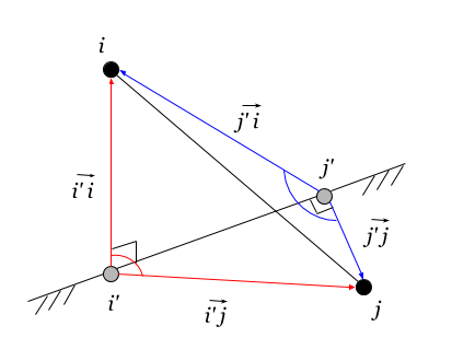
If the vertices do not belong to the base space (belong to the superspace), then two situations are possible:
1. Vertices belong to the same (above) space. In this case, the vertices and their projections onto the base space lie in the same plane.
2. Vertices belong to different (above) spaces (shown in the figure above).
In the first situation, the direction of the normals vecai and vecaj collinear, so the scalar product coincides with the product of the distances from the vertices to the base space:
Fij= sqrtNiNj quad(4.6.3)
The sign of the square root is positive if the vertices are on the same side of space (the normals are directed to one side) and negative in the opposite case. This formula has already been cited in the 2nd article of the series - (2.7) . Formula (4.6.3) describes a particular (albeit important) case.
To build a coordinate system, it is necessary to determine the scalar component of the bi-coordinates - what is called the orbital of the element . Without this component, the distances in the graph can be obtained only within the framework of the base space.
For determining the bi-coordinates , a formula was obtained linking the orbital of the element and its projection onto the basis space with the norm of the element - (2.9.1):
Wt=Wt′+Nt/2 quad(4.7)
The orbital of the projection of an element can be calculated through the bilinear form (2.9.2), since we know it as the Gramian of the basis Gaa and barycentric coordinates of elements (4.4.3). The values of the norms of elements according to (4.6.2) can be taken from the diagonal elements of the fundamental matrix. Putting it all together, we get an expression for the matrix of mutual orbitals:
Wtt=−(Bat Gaa Bat+Ftt)/2 quad(4.8)
Diagonal values of this matrix Diag(wtt) - these are orbitals of vertices.
Thus, the bi-coordinates of the outer vertices are defined. Based on the bi-coordinates, it is possible to calculate the di-coordinates using the formula (4.4.4), to obtain the mutual norms matrix (4.4.2).
The task of building a coordinate system is completed.
If the basis contains a small number of vertices, then part of the inversion formulas (4.4) can be expressed explicitly. Here we consider the bases of one and two vertices.
Quite trivial and therefore not very interesting. The remote metric tensor of the basis does not include a single distance:
Gm = \ begin {pmatrix} 0 & 1 \\ 1 & 0 \ end {pmatrix}
All barycentric coordinates of the vertices with respect to the base are equal to 1 (since there is only one component). The fundamental matrix coincides with the matrix of scalar products of pairs, where the first element of each pair is just the vertex of the base. In the 3rd part it was shown that the distance matrix on the basis of such a matrix can be obtained through distance conversion :
Qij=Fii+Fjj−2Fij
Such a basis has practical value. For example, in the electrometry problem we considered earlier, the nodes to which an external voltage is applied are the 2-vertex basis.
Denote the distance between the base vertices A and B as r=qAB . Recall that in an electrical circuit the distance is equivalent to the resistance between the nodes. Then the remote metric base tensor is:
Gm = \ begin {pmatrix} 0 & 1 & 1 \\ 1 & 0 & -r / 2 \\ 1 & -r / 2 & 0 \ end {pmatrix} \ quad (4.9)
Determinant of DMT: Det(Gm)=−r . Laplace tensor (LMT) is obtained by addressing the remote (4.4.1):
Lm = \ begin {pmatrix} r / 4 & 0.5 & 0.5 \ 0.5 & / r & - / r \\ 0.5 & - / r & / r \ end {pmatrix} \ quad (4.10)
Di-coordinates of the graph vertices will have three components: scalar (1), scalar products dA relative to the base vertex A and dot products dB relative to the base vertex B :
Dm=[1;dA,dB] quad(4.11.1)
The bi-coordinates also have three components. The scalar component is the (geometric) vertex orbital.
Bm=[w;B]=[w;bA,bB] quad(4.11.2)
Substituting (4.11.1) into (4.4.5) and taking into account (3.8), we obtain expressions for the components of the bi-coordinates of the vertex P :
BmP=[−gPAB/2;gBAP/r,gABP/r] quad(4.12)
Here through gZXY=gZX,ZY denotes the scalar product of pairs whose beginning is at the vertex Z , and the ends - in the elements X and Y .
gZXY=dXY−dXZ−dYZ quad(4.13)
You can make sure that the sum of the barycentric components is equal to 1, as it should be: bA+bB=1 .
The barycentric part of the coordinates in (4.12) is an influence matrix - it transmits the influence of the base vertices on the external ones. If, for example, the values of the potentials are given on the base vertices Ua , then the potentials of the other vertices Ut determined by the product of the specified potentials on the matrix of influence:
UP=BaPUa quad(4.14)
Let the vector of given potentials be Ua=[UA,0] . Then the potential difference between the elements P and Q of the graph will be equal to:
U P - U Q = ( B P A - B Q A ) U A = g A B , P Q U A / r = g A B , P Q J q u a d ( 4.15 ) In the derivation used identity (3.9. 4) for the difference of the scalar products of adjacent pairs.
J is the value of the incoming flow, is determined by the equationL a U a = J .
Formula (4.15) explicitly expresses the connection of the potential differences at the vertices of the graph with the scalar product, which was indicated in the previous article .
Let's sum up.This part shows how to set the coordinate system on the graph. The basic identities are given, the key ones of which, in our opinion, are (4.5) and (4.5.1).
From the obligatory program, it remains to consider the coordinate transformation (change of the basis), and this will be dealt with in the next article .
Table of contents
What is graph space
The dimension of space and the dimension of the basis
The dimension of the space of a graph is determined by the number of its connected vertices (we will assume that all the vertices of the graph are connected — a one-component graph). The basis of space is defined as a subset of the vertices of the graph with known distances between them (the metric). A subset may include all the vertices of the graph, or only a part (subgraph). In the latter case, the basis dimension is less than the dimension of the general space of the graph.
Elements in graph space
It is necessary to understand what are the elements and vectors on the graph. A graph is a set of related elements (nodes). The nodes of the graph determine its set of potential basic elements, and the connections - the metric, the distance between the basic elements.
As a basis for determining the coordinate system on a graph, not all nodes of the graph can be selected, but only a part of it - the base subgraph. In this case, the total space of the graph can be divided into two subspaces - basic and outside basic (external).
')
The nodes that are included in the basis of the graph are called basic. All other space elements are set relative to its base nodes through the barycentric coordinates (weights of the base vertices).
In the general case, an element can either belong to the space of a basis, or lie outside its limits. Elements outside the base will be called external . Since the outer element has a nonzero distance to the base space, each outer element is a graph node that is not included in its basis. That is, the external elements are explicitly specified in the structure of the graph.
The elements belonging to the space of a basis do not appear in any way in the structure - virtual elements (except for the directly defined vertices of the basis). The rate of virtual elements is zero — it is simply the vector of potentials normalized to unity at the vertices of the basis. An example of a virtual basis space element is the center of the described sphere.
If the graph is an electrical circuit, then the element is the set of potentials at the nodes of the network. The Laplacian of an electrical circuit is a matrix consisting of the conductivities of the ribs. Multiplying this matrix by the electrical potentials of the nodes gives the current in the nodes. Accordingly, the potentials at the nodes are the distance coordinates. u i e q u i v d m i , and the total node current is barycentric: i j e q u i v b m j . Coordinate transformation simply reflects Ohm’s law :
L j i u i = i j
In contrast to the usual perception of space, in which elements are something material, and their components are virtual (weights, distances, projections), the situation in the graph space is reversed. The components of the element (potentials and currents in the nodes) are material, and the position of the element in space is virtually virtual and is determined by the totality of the component values.
Building a coordinate system on a graph
Formulation of the problem
The task of building a coordinate system (SC) on a graph can be formulated as follows.
- A graph is defined as a set of interconnected vertices.
- From the set of all vertices of the graph, a basis is selected — a set of vertices for which you can construct a metric tensor — distance or Laplace.
- The remaining vertices of the graph are external. For external vertices are known:
- The total connectivity of a vertex (the sum of the weights of its connections).
- Connections between vertices.
- Connections of external vertices with vertices of a basis.
It is required to determine the coordinates of the outer vertices relative to the base. The coordinate system should allow to determine the distance between all (any) vertices of the graph.
We clarify that only one of the possible formulations of the problem of constructing a CS is given. Combinations of known parameters and those that need to be determined may vary.
Basic subgraph
Denote the set of base vertices of the graph by the index a (anchor-anchor), and the set of the remaining vertices by the index t . Combining these sets gives all the vertices of the graph. We consider the nodes of the graph connected with the rest at least one bond.
General distance metric tensor (DMT) graph G m can be divided into 4 matrices:
Gm = \ begin {pmatrix} Gm_ {aa} & Dm_ {at} \\ Dm_ {ta} & G_ {tt} \ end {pmatrix} \ quad (4.1.1)Gm = \ begin {pmatrix} Gm_ {aa} & Dm_ {at} \\ Dm_ {ta} & G_ {tt} \ end {pmatrix} \ quad (4.1.1)
G m a a - remote metric tensor of a subgraph;
D m a t - di-coordinate matrix of external vertices t in basis a . In this matrix, the coordinates of the vertex are the column of the matrix in the transposed D m t a - line.
G t t - matrix of scalar products between the vertices of the graph that are not included in the basis.
Under the conditions of the problem, only the Gramian of a subgraph is known. G m a a . Matrices D m a t and G t t - this is what must be determined on the basis of data on the structure of the graph.
Structure of the laplacian
In the same way (into 4 submatrices) the Laplacian of the graph can be broken L . Unlike the Gramian, the Laplacian of the graph is minor here - data on the basis sphere of the graph are absent.
L = \ begin {pmatrix} L ^ {aa} & -C ^ {at} \\ -C ^ {ta} & L ^ {tt} \ end {pmatrix} \ quad (4.1.2)L = \ begin {pmatrix} L ^ {aa} & -C ^ {at} \\ -C ^ {ta} & L ^ {tt} \ end {pmatrix} \ quad (4.1.2)
Cat=−Lat - matrix of connections (adjacency) between the outer vertices of the graph t and its basis a .
Ltt - Laplacian minor, connections of external vertices. On the diagonal of this matrix are the values of the total conductivity of the node (the total weight of its edges), the remaining elements - the magnitude of the connection of the nodes between them. This matrix is usually reversible. Its appeal is called the fundamental matrix :
Ftt=/Ltt quad(4.2)
The term "fundamental" is taken from the theory of Markov chains with absorption. In such circuits, the role of base is played by nodes from which there is no return (absorbing). An example of the use of this matrix was given in the article about the method of ranking objects according to their degree of distance from the given ones.
It is assumed that one of the matrices (Laplacian minor Ltt or fundamental matrix Ftt ) are known. According to (4.2), one can express one of the other.
Basic identities
Gramihan and Laplacian graph are mutually inverse.
Gm cdotLm=I quad(4.3)
To find the identities connecting the matrices listed above, it is necessary to substitute the block matrices (4.1.1) and (4.1.2) into (4.3) (the Laplacian is preliminarily edged with conditional parameters of the basis sphere). As a result, we obtain the following relations.
Laplace communication Lmaa and remote Gmaa metric tensors of subgraph basis:
LmaaGmaa=Iaa quad(4.4.1)
(4.4.1) allows us to calculate one tensor based on the other. If the basis is specified in the form of links, then to determine the basis Laplacian La You can use the following identity:
La=Laa−BatCta=Laa−CatFttCta quad(4.4.2)
Here Laa - minor of the original Laplacian on the basic vertices. La - Laplacian, submatrix of LMT basis. Based on this Laplacian, you can find the Grammian subgraph Gmaa .
If the matrix of relations between external nodes of the graph and its basis is known Cat as well as the fundamental matrix Ftt , it is possible to calculate the barycentric coordinates of the nodes:
Bat=CatFtt quad(4.4.3)
Matrix of barycentric coordinates Bat also called the influence matrix . Indeed, its values reflect the influence of the base vertices on the others (in the Dirichlet problem, the influence of the values of the boundary nodes on the external ones).
The bi- and di-coordinates of the nodes are mutual. Expressed through the metric basis tensor:
Dmat=GmaaBmat, quadBmat=LmaaDmat quad(4.4.4)
Di-coordinates include the unit and the values of scalar products of elements with a basis: Dmta=[1t;Dta] .
Bi-coordinates consist of a scalar component (orbitals) and barycentric coordinates:
Bmat=[Wt;Bat]
If the determinants of the fundamental matrix and the LMT basis are known, then the total scalar potential of the Laplacian of the graph can be calculated:
u(L)=−Det(Lmaa)/Det(Ftt) quad(4.4.5)
Matrix of scalar products of external vertices Gatt in subgraph basis a is a bilinear form, expressed in terms of bi- or di-coordinates of vertices:
Gatt=DmtaLmaaDmat=BmatGmaaBmat quad(4.4.6)
The fundamental matrix and the distance between the vertices
Obviously, the values of the matrix Gatt will generally differ from the scalar products of the vertices in the original graph Gtt . The difference between them is expressed by the fundamental matrix:
Gtt−Gatt=Ftt quad(4.5)
Formula (4.5) can be used to calculate the true scalar product between vertices (elements) Gtt if scalar product of elements is known in the basis of a subgraph Gatt and the fundamental matrix Ftt .
In the original graph, the norms of the vertices are zero. Accordingly, the dot product Gtt can be expressed in terms of the square of the distance between the vertices Qtt : Gtt=−Qtt/2 . Then (4.5) can be represented as:
Ftt+Gatt+Qtt/2=0 quad(4.5.1)
With this expression, we have already met in the 2nd part in determining the scalar product of elements - (2.6) . Comparing expressions, we see that the values of the fundamental matrix can be expressed in terms of the scalar product of the vertices with respect to the basis:
Fij=Gii′,jj′=Gij,a=−(Qij+Qi′j′−Qij′−Qi′j)/2 quad(4.6.1)
The strokes mark the projections of the vertices onto the base space. Gii′,jj′ Is a scalar product of pairs (i,i′) and (j,j′) .
Through Gij,a denotes the scalar product of vertex normals i,j to space a .
The normal is defined as the direction from the element to its projection in the basis space. This is close to the definition of the scalar product of the coordinates of elements in ordinary coordinate systems (on a vector basis), but instead of the origin, the space is indicated here.
If any of the vertices belongs to a basis space, then its scalar product with respect to a basis with any other vertex is zero. Thus, if one of the elements of the fundamental matrix is zero, then the entire row and column of the matrix will also be zero.
If items i and j coincide, the value of the fundamental matrix is equal to the distance from the element to the base space or according to (2.5) the negative element norm
Fii=−Ni quad(4.6.2) - the values of the diagonal elements of the fundamental matrix.
Distances between elements outside the basis space
If the vertices do not belong to the base space (belong to the superspace), then two situations are possible:
1. Vertices belong to the same (above) space. In this case, the vertices and their projections onto the base space lie in the same plane.
2. Vertices belong to different (above) spaces (shown in the figure above).
In the first situation, the direction of the normals vecai and vecaj collinear, so the scalar product coincides with the product of the distances from the vertices to the base space:
Fij= sqrtNiNj quad(4.6.3)
The sign of the square root is positive if the vertices are on the same side of space (the normals are directed to one side) and negative in the opposite case. This formula has already been cited in the 2nd article of the series - (2.7) . Formula (4.6.3) describes a particular (albeit important) case.
Matrix orbitals
To build a coordinate system, it is necessary to determine the scalar component of the bi-coordinates - what is called the orbital of the element . Without this component, the distances in the graph can be obtained only within the framework of the base space.
For determining the bi-coordinates , a formula was obtained linking the orbital of the element and its projection onto the basis space with the norm of the element - (2.9.1):
Wt=Wt′+Nt/2 quad(4.7)
The orbital of the projection of an element can be calculated through the bilinear form (2.9.2), since we know it as the Gramian of the basis Gaa and barycentric coordinates of elements (4.4.3). The values of the norms of elements according to (4.6.2) can be taken from the diagonal elements of the fundamental matrix. Putting it all together, we get an expression for the matrix of mutual orbitals:
Wtt=−(Bat Gaa Bat+Ftt)/2 quad(4.8)
Diagonal values of this matrix Diag(wtt) - these are orbitals of vertices.
Thus, the bi-coordinates of the outer vertices are defined. Based on the bi-coordinates, it is possible to calculate the di-coordinates using the formula (4.4.4), to obtain the mutual norms matrix (4.4.2).
The task of building a coordinate system is completed.
An example of building a coordinate system
Let us turn to the graph presented at the KDPV. It has three basic vertices - 1, 2 and 5. It is required to determine the coordinates of the remaining outer vertices - 3, 4 and 6.
The vertices of the base could be any, including not connected to each other. A good basis is the vertices with the highest connectivity (in our graph, these are the vertices 2, 4, 5). With such a basis, the remaining vertices are weakly interconnected. The minor of the Laplacian and the fundamental matrix are diagonal (no connections) and everything is simplified. But we are interested in the general case in which there are links between external vertices.
Laplacian:
\ begin {array} {c | ccc with cc}
L & 1 & 2 & 3 & 4 & 5 & 6
\ hline
1 & 2 & -1 & 0 & 0 & -1 & 0 \\
2 & -1 & 3 & -1 & 0 & -1 & 0 \\
3 & 0 & -1 & 2 & -1 & 0 & 0 \\
4 & 0 & 0 & -1 & 3 & -1 & -1 \\
5 & -1 & -1 & 0 & -1 & 3 & 0 \\
6 & 0 & 0 & 0 & -1 & 0 & 1 \\
\ end {array}
Corresponding distance matrix:
\ begin {array} {c | ccc with cc}
Q & 1 & 2 & 3 & 4 & 5 & 6 \\
\ hline
1 & 0 & 0. (63) & 1. (18) & 1. (18) & 0. (63) & 2. (18) \\
2 & 0. (63) & 0 & 0. (72) & 0. (90) & 0. (54) & 1. (90) \\
3 & 1. (18) & 0. (72) & 0 & 0. (72) & 0.909 & 1. (72) \\
4 & 1. (18) & 0. (90) & 0. (72) & 0 & 0. (72) & 1.00 \\
5 & 0. (63) & 0. (54) & 0. (90) & 0. (72) & 0 & 1. (72) \\
6 & 2. (18) & 1. (90) & 1. (72) & 1.00 & 1. (72) & 0 \\
\ end {array}
Gramihan (distance metric tensor) basis G m a a will be of the form (data taken from the general distance matrix of the graph and divided by -2):
\ begin {array} {c | ccc with}
Gm_ {aa} & 0 & 1 & 2 & 5 \\
\ hline
0 & 0 & 1 & 1 & 1 \\
1 & 1 & 0 & -0.3 (18) & -0.3 (18) \\
2 & 1 & -0.3 (18) & 0 & -0. (27) \\
5 & 1 & -0.3 (18) & -0. (27) & 0 \\
\ end {array}
The adjacency matrix (relations with the base) C a t in our example, it looks like:
\ begin {array} {c | ccc}
C ^ {at} & 3 & 4 & 6 \\
\ hline
1 & 0 & 0 & 0 \\
2 & 1 & 0 & 0 \\
5 & 0 & 1 & 0 \\
\ end {array}
We see that the 3rd vertex is connected with the 2nd vertex of the base, and the 4th vertex is with the 5th vertex. The 6th vertex is not connected with a basis.
Minor Laplacian External Relations Ltt will be like this:
\ begin {array} {c | ccc}
L ^ {tt} & 3 & 4 & 6 \\
\ hline
3 & 2 & -1 & 0 \\
4 & -1 & 3 & -1 \\
6 & 0 & -1 & 1 \\
\ end {array}
Baseline triad Gmaa,Cat,Ltt - set. Based on the matrix data, you can restore all the parameters of the original graph.
Paying laplacian minor Ltt , we obtain the values of the fundamental matrix Ftt (4.2):
\ begin {array} {c | ccc}
F_ {tt} & 3 & 4 & 6 \\
\ hline
3 & 2/3 & 1/3 & 1/3 \\
4 & 1/3 & 2/3 & 2/3 \\
6 & 1/3 & 2/3 & 5/3 \\
\ end {array}
Barycentric coordinates of external vertices Bat we obtain by the formula (4.4.3):
\ begin {array} {c | ccc}
B ^ {a} _ {t} & 3 & 4 & 6 \\
\ hline
1 & 0 & 0 & 0 \\
2 & 2/3 & 1/3 & 1/3 \\
5 & 1/3 & 2/3 & 2/3 \\
\ end {array}
We see that the barycentric coordinates of vertex 6 coincide with the barycentric coordinates of node 4. This is typical for all nodes that are connected to only one vertex. Geometrically, this means that the projections of nodes 6 and 4 onto the space of a basis coincide.
In all vertices of the component, the base vertex 1 is zero. That is, the contribution to the barycentric coordinates of the vertices of the graph is made only by the vertices that are associated with them - the outer vertices of the base subgraph.
Mutual orbitals matrix Wtt calculated on the basis of barycentric coordinates and the fundamental matrix (4.8):
\ begin {array} {c | ccc}
W_ {tt} & 3 & 4 & 6 \\
\ hline
3 & 0. (54) & 0. (18) & 0. (18) \\
4 & 0. (18) & 0. (54) & 0. (54) \\
6 & 0. (18) & 0. (54) & 1. (54) \\
\ end {array}
Now you can build bi-coordinates of elements. Bmat - the scalar component is equal to the diagonal values of the matrix of the orbitals, divided by (-2):
\ begin {array} {c | ccc}
Bm ^ {a} _ {t} & 3 & 4 & 6 \\
\ hline
0 & -0. (27) & -0. (27) & -0.7 (72) \\
1 & 0 & 0 & 0 \\
2 & 0. (6) & 0. (3) & 0. (3) \\
5 & 0. (3) & 0. (6) & 0. (6) \\
\ end {array}
Multiplying the matrix of the bi-coordinates by the base grammian, we get the di-coordinates Dmat .
\ begin {array} {c | ccc}
Dm_ {at} & 3 & 4 & 6 \\
\ hline
0 & 1 & 1 & 1 \\
1 & -0.5 (90) & -0.5 (90) & -1. (09) \\
2 & -0. (36) & -0. (45) & -0.9 (54) \\
5 & -0. (45) & -0. (36) & -0.8 (63) \\
\ end {array}
The distance between the vertices of the graph 6 and 1 according to this matrix should be equal to Q16=2 cdot1.(09)=2.(18) . Looking at the total distance matrix, you can make sure that it is.
Matrix of scalar products in a subgraph Gatt - this is the product of the mutual coordinates of the vertices:
\ begin {array} {c | ccc}
N_ {tt} & 3 & 4 & 6 \\
\ hline
3 & -0. (6) & -0. (69) & -1.1 (96) \\
4 & -0. (69) & -0. (6) & -1.1 (6) \\
6 & -1.1 (96) & -1.1 (6) & -1. (6) \\
\ end {array}
According to this matrix, all external vertices of the graph lie outside the base space (the norms are nonzero). It remains to determine the distance between the outer peaks. Qtt . Use (4.5 '):
\ begin {array} {c | ccc}
Q_ {tt} & 3 & 4 & 6 \\
\ hline
3 & 0 & 0. (72) & 1. (72) \\
4 & 0. (72) & 0 & 1.0 \\
6 & 1. (72) & 1.0 & 0 \\
\ end {array}
Compare with the original distance matrix Q and make sure all values match.
Graph of 6 vertices with a basis of 3
Let us turn to the graph presented at the KDPV. It has three basic vertices - 1, 2 and 5. It is required to determine the coordinates of the remaining outer vertices - 3, 4 and 6.
The vertices of the base could be any, including not connected to each other. A good basis is the vertices with the highest connectivity (in our graph, these are the vertices 2, 4, 5). With such a basis, the remaining vertices are weakly interconnected. The minor of the Laplacian and the fundamental matrix are diagonal (no connections) and everything is simplified. But we are interested in the general case in which there are links between external vertices.
Source graph - for verification
Laplacian:
\ begin {array} {c | ccc with cc}
L & 1 & 2 & 3 & 4 & 5 & 6
\ hline
1 & 2 & -1 & 0 & 0 & -1 & 0 \\
2 & -1 & 3 & -1 & 0 & -1 & 0 \\
3 & 0 & -1 & 2 & -1 & 0 & 0 \\
4 & 0 & 0 & -1 & 3 & -1 & -1 \\
5 & -1 & -1 & 0 & -1 & 3 & 0 \\
6 & 0 & 0 & 0 & -1 & 0 & 1 \\
\ end {array}
Corresponding distance matrix:
\ begin {array} {c | ccc with cc}
Q & 1 & 2 & 3 & 4 & 5 & 6 \\
\ hline
1 & 0 & 0. (63) & 1. (18) & 1. (18) & 0. (63) & 2. (18) \\
2 & 0. (63) & 0 & 0. (72) & 0. (90) & 0. (54) & 1. (90) \\
3 & 1. (18) & 0. (72) & 0 & 0. (72) & 0.909 & 1. (72) \\
4 & 1. (18) & 0. (90) & 0. (72) & 0 & 0. (72) & 1.00 \\
5 & 0. (63) & 0. (54) & 0. (90) & 0. (72) & 0 & 1. (72) \\
6 & 2. (18) & 1. (90) & 1. (72) & 1.00 & 1. (72) & 0 \\
\ end {array}
Input data
Gramihan (distance metric tensor) basis G m a a will be of the form (data taken from the general distance matrix of the graph and divided by -2):
\ begin {array} {c | ccc with}
Gm_ {aa} & 0 & 1 & 2 & 5 \\
\ hline
0 & 0 & 1 & 1 & 1 \\
1 & 1 & 0 & -0.3 (18) & -0.3 (18) \\
2 & 1 & -0.3 (18) & 0 & -0. (27) \\
5 & 1 & -0.3 (18) & -0. (27) & 0 \\
\ end {array}
The adjacency matrix (relations with the base) C a t in our example, it looks like:
\ begin {array} {c | ccc}
C ^ {at} & 3 & 4 & 6 \\
\ hline
1 & 0 & 0 & 0 \\
2 & 1 & 0 & 0 \\
5 & 0 & 1 & 0 \\
\ end {array}
We see that the 3rd vertex is connected with the 2nd vertex of the base, and the 4th vertex is with the 5th vertex. The 6th vertex is not connected with a basis.
Minor Laplacian External Relations Ltt will be like this:
\ begin {array} {c | ccc}
L ^ {tt} & 3 & 4 & 6 \\
\ hline
3 & 2 & -1 & 0 \\
4 & -1 & 3 & -1 \\
6 & 0 & -1 & 1 \\
\ end {array}
Baseline triad Gmaa,Cat,Ltt - set. Based on the matrix data, you can restore all the parameters of the original graph.
Restore graph
Paying laplacian minor Ltt , we obtain the values of the fundamental matrix Ftt (4.2):
\ begin {array} {c | ccc}
F_ {tt} & 3 & 4 & 6 \\
\ hline
3 & 2/3 & 1/3 & 1/3 \\
4 & 1/3 & 2/3 & 2/3 \\
6 & 1/3 & 2/3 & 5/3 \\
\ end {array}
Barycentric coordinates of external vertices Bat we obtain by the formula (4.4.3):
\ begin {array} {c | ccc}
B ^ {a} _ {t} & 3 & 4 & 6 \\
\ hline
1 & 0 & 0 & 0 \\
2 & 2/3 & 1/3 & 1/3 \\
5 & 1/3 & 2/3 & 2/3 \\
\ end {array}
We see that the barycentric coordinates of vertex 6 coincide with the barycentric coordinates of node 4. This is typical for all nodes that are connected to only one vertex. Geometrically, this means that the projections of nodes 6 and 4 onto the space of a basis coincide.
In all vertices of the component, the base vertex 1 is zero. That is, the contribution to the barycentric coordinates of the vertices of the graph is made only by the vertices that are associated with them - the outer vertices of the base subgraph.
Mutual orbitals matrix Wtt calculated on the basis of barycentric coordinates and the fundamental matrix (4.8):
\ begin {array} {c | ccc}
W_ {tt} & 3 & 4 & 6 \\
\ hline
3 & 0. (54) & 0. (18) & 0. (18) \\
4 & 0. (18) & 0. (54) & 0. (54) \\
6 & 0. (18) & 0. (54) & 1. (54) \\
\ end {array}
Now you can build bi-coordinates of elements. Bmat - the scalar component is equal to the diagonal values of the matrix of the orbitals, divided by (-2):
\ begin {array} {c | ccc}
Bm ^ {a} _ {t} & 3 & 4 & 6 \\
\ hline
0 & -0. (27) & -0. (27) & -0.7 (72) \\
1 & 0 & 0 & 0 \\
2 & 0. (6) & 0. (3) & 0. (3) \\
5 & 0. (3) & 0. (6) & 0. (6) \\
\ end {array}
Multiplying the matrix of the bi-coordinates by the base grammian, we get the di-coordinates Dmat .
\ begin {array} {c | ccc}
Dm_ {at} & 3 & 4 & 6 \\
\ hline
0 & 1 & 1 & 1 \\
1 & -0.5 (90) & -0.5 (90) & -1. (09) \\
2 & -0. (36) & -0. (45) & -0.9 (54) \\
5 & -0. (45) & -0. (36) & -0.8 (63) \\
\ end {array}
The distance between the vertices of the graph 6 and 1 according to this matrix should be equal to Q16=2 cdot1.(09)=2.(18) . Looking at the total distance matrix, you can make sure that it is.
Matrix of scalar products in a subgraph Gatt - this is the product of the mutual coordinates of the vertices:
\ begin {array} {c | ccc}
N_ {tt} & 3 & 4 & 6 \\
\ hline
3 & -0. (6) & -0. (69) & -1.1 (96) \\
4 & -0. (69) & -0. (6) & -1.1 (6) \\
6 & -1.1 (96) & -1.1 (6) & -1. (6) \\
\ end {array}
According to this matrix, all external vertices of the graph lie outside the base space (the norms are nonzero). It remains to determine the distance between the outer peaks. Qtt . Use (4.5 '):
\ begin {array} {c | ccc}
Q_ {tt} & 3 & 4 & 6 \\
\ hline
3 & 0 & 0. (72) & 1. (72) \\
4 & 0. (72) & 0 & 1.0 \\
6 & 1. (72) & 1.0 & 0 \\
\ end {array}
Compare with the original distance matrix Q and make sure all values match.
Minor-vertex bases
If the basis contains a small number of vertices, then part of the inversion formulas (4.4) can be expressed explicitly. Here we consider the bases of one and two vertices.
Basis from one vertex
Quite trivial and therefore not very interesting. The remote metric tensor of the basis does not include a single distance:
Gm = \ begin {pmatrix} 0 & 1 \\ 1 & 0 \ end {pmatrix}
All barycentric coordinates of the vertices with respect to the base are equal to 1 (since there is only one component). The fundamental matrix coincides with the matrix of scalar products of pairs, where the first element of each pair is just the vertex of the base. In the 3rd part it was shown that the distance matrix on the basis of such a matrix can be obtained through distance conversion :
Qij=Fii+Fjj−2Fij
Two vertex basis
Such a basis has practical value. For example, in the electrometry problem we considered earlier, the nodes to which an external voltage is applied are the 2-vertex basis.
Denote the distance between the base vertices A and B as r=qAB . Recall that in an electrical circuit the distance is equivalent to the resistance between the nodes. Then the remote metric base tensor is:
Gm = \ begin {pmatrix} 0 & 1 & 1 \\ 1 & 0 & -r / 2 \\ 1 & -r / 2 & 0 \ end {pmatrix} \ quad (4.9)
Determinant of DMT: Det(Gm)=−r . Laplace tensor (LMT) is obtained by addressing the remote (4.4.1):
Lm = \ begin {pmatrix} r / 4 & 0.5 & 0.5 \ 0.5 & / r & - / r \\ 0.5 & - / r & / r \ end {pmatrix} \ quad (4.10)
Di-coordinates of the graph vertices will have three components: scalar (1), scalar products dA relative to the base vertex A and dot products dB relative to the base vertex B :
Dm=[1;dA,dB] quad(4.11.1)
The bi-coordinates also have three components. The scalar component is the (geometric) vertex orbital.
Bm=[w;B]=[w;bA,bB] quad(4.11.2)
Substituting (4.11.1) into (4.4.5) and taking into account (3.8), we obtain expressions for the components of the bi-coordinates of the vertex P :
BmP=[−gPAB/2;gBAP/r,gABP/r] quad(4.12)
Here through gZXY=gZX,ZY denotes the scalar product of pairs whose beginning is at the vertex Z , and the ends - in the elements X and Y .
gZXY=dXY−dXZ−dYZ quad(4.13)
You can make sure that the sum of the barycentric components is equal to 1, as it should be: bA+bB=1 .
The potential difference of the graph with a 2-vertex basis
The barycentric part of the coordinates in (4.12) is an influence matrix - it transmits the influence of the base vertices on the external ones. If, for example, the values of the potentials are given on the base vertices Ua , then the potentials of the other vertices Ut determined by the product of the specified potentials on the matrix of influence:
UP=BaPUa quad(4.14)
Let the vector of given potentials be Ua=[UA,0] . Then the potential difference between the elements P and Q of the graph will be equal to:
U P - U Q = ( B P A - B Q A ) U A = g A B , P Q U A / r = g A B , P Q J q u a d ( 4.15 ) In the derivation used identity (3.9. 4) for the difference of the scalar products of adjacent pairs.
J is the value of the incoming flow, is determined by the equationL a U a = J .
Formula (4.15) explicitly expresses the connection of the potential differences at the vertices of the graph with the scalar product, which was indicated in the previous article .
Let's sum up.This part shows how to set the coordinate system on the graph. The basic identities are given, the key ones of which, in our opinion, are (4.5) and (4.5.1).
From the obligatory program, it remains to consider the coordinate transformation (change of the basis), and this will be dealt with in the next article .
Source: https://habr.com/ru/post/339672/
All Articles