Traffic Sign Recognition Using CNN: Spatial Transformer Networks
Hi, Habr! We continue a series of materials from a graduate of our program Deep Learning, Cyril Danilyuk, on the use of convolutional neural networks for pattern recognition - CNN (Convolutional Neural Networks).
In the last post, we started talking about preparing data for training a convolutional network. Now is the time to use the data and try to build on them the neural network classifier of road signs. This is what we will do in this article, adding in addition to the classifier network a curious module - STN. Dataset we use the same as before .
Spatial Transformer Network (STN) is one of the examples of differentiable LEGO-modules, on the basis of which you can build and improve your neural network. STN, applying a learning affine transform followed by interpolation, deprives images of spatial invariance. Roughly speaking, the task of STN is to rotate or reduce-enlarge the original image so that the main classifier network can more easily determine the desired object. The STN block can be placed on a convolutional neural network (CNN), working for the most part on its own, learning from gradients coming from the main network.
')
All project source code is available on GitHub by reference . The original of this article can be viewed at Medium .
To have a basic understanding of how STN works, take a look at 2 examples below:
 Left: the original image. Right: the same image converted by STN. The spatial transformers recognize the most important part of the image and then scale or rotate it to focus on that part.
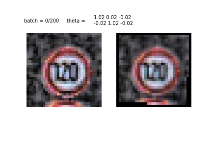
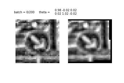
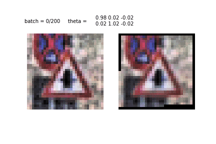 Another example of STN training and image conversion. This is the first era and the first tens of batches used for training. It can be seen how the STN recognizes the shape of the sign, to then concentrate on it.
STN works even in difficult cases (for example, 2 characters in the image), but most importantly, STN really improves the quality of the classifier (IDSIA in my case).
One of the problems of convolutional neural networks is that the invariance to the input data is too low: different scale, point of shooting, background noise and much more . You can, of course, say that the pooling operation, so not favored by Hinton, gives some invariance, but in fact it simply reduces the size of the feature map, which results in the loss of information.
Unfortunately, due to the small receptive field in the standard 2x2 pooling, spatial invariance can only be achieved in deep layers close to the output layer. Also, pooling does not provide the invariance of rotation and scale. Kevin Zakka well explained the reason for this in his post .
The main and most common way to make the model resistant to these variations is dataset augmentation, which we did in the previous article :
Augmented images. In this post we will not use augmentation.
There is nothing wrong with this approach, but we would like to develop a smarter and more automated method for image preprocessing, which should help increase the accuracy of the classifier. Spatial transformer network (STN) - just what we need.
Below is another example of how STN works:
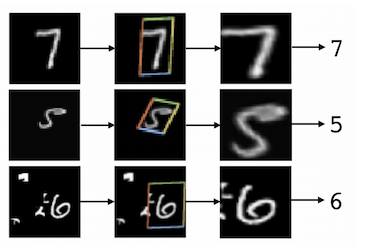
An example from the MNIST dataset from the original article. Cluttered MNIST (left), target, recognized STN (center), transformed image (right).
The work of the STN module can be reduced to the following process (not including training):
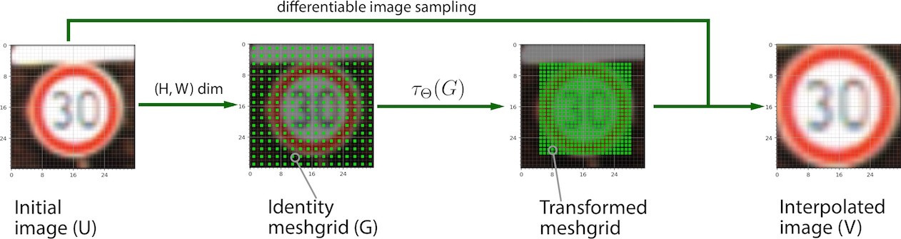
Application of STN conversion in 4 steps with a known matrix of linear transformations θ .
Now let's take a closer look at this process and each of its stages.
Step 1. Determine the transformation matrix θ , which describes the transformation itself:
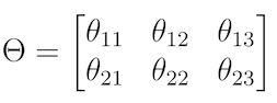
Affine transformation of the matrix θ .
Moreover, each transformation corresponds to its own matrix. We are interested in the following 4:
Step 2. Instead of applying the transform directly to the source image ( U ), create a sampling meshgrid of the same size as U. The sample grid is a set of indices (x_t, y_t) that cover the original image space. The grid does not contain any information about the color of the images. This is better explained in the code below:
Since this is the actual implementation in TensorFlow, in order to understand the general idea, we will translate this code into an analogue of numpy:
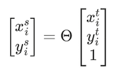
Step 3. Apply a linear transformation matrix to the created sample grid to get a new set of points on the grid, each of which can be defined as the result of multiplying the matrix θ by the coordinate vector (x_t, y_t) with a free member:
Step 4. Obtain subsample V using the original feature map, transformed sample grid (see Step 3) and a differentiated interpolation function of your choice (for example, bilinear). Interpolation is necessary because we need to translate the result of the sampling (potentially possible fractional pixel values) into whole numbers.
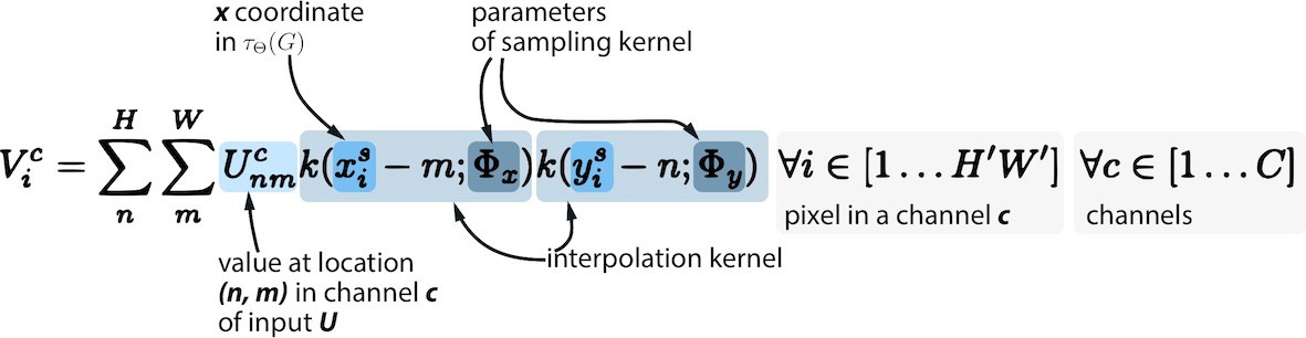
Sampling and interpolation
The task of learning . Generally speaking, if we knew in advance the necessary θ values for each source image, we could begin the process described above. In fact, we would like to extract θ from the data using machine learning. This is quite realistic. First , we need to make sure that the loss function of the road sign classifier can be minimized using backprop through the sampler. Secondly , we find gradients in U and G (meshgrid): this is why the interpolation function must be differentiable or, at least, partially differentiable. Third , we calculate the partial derivatives of x and y with respect to θ . Technical calculations can be read in the original paper.
Finally, we create LocNet (a localizing network-regressor) , the only task of which is to train and predict the correct θ for the input image using the loss function, which was minimized through total backprop.
The main advantage of this approach is that we get a differentiable stand-alone module with memory (in the form of trained weights), which can be placed in any part of CNN.
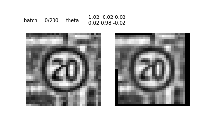
Notice how θ changes as STN learns to recognize the target object (road sign) in the images.
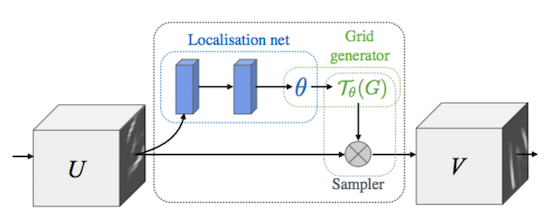
Below is a diagram of the STN from the original article:
We reviewed all the steps involved in building an STN: the creation of LocNet, a sample mesh generator (meshgrid) and a sampler. Now we will build and train on TensorFlow the entire classifier, which includes in its graph and STN.
The entire model code, of course, does not fit into the framework of a single article, but it is available as a Jupyter laptop in the repository on GitHub .
In this article, I focus on some important parts of the code and the stages of learning the model.
First, our ultimate goal is to learn to recognize road signs, and to achieve it we need to create some kind of classifier and train it. We have many options: from LeNet to any other SOTA-neural network. In the process of working on the project, inspired by the work of Moodstocks on STN (implemented in Torch), I used the IDSIA neural network architecture, although nothing prevented me from taking something else.
At the second stage, we need to identify and train the STN module, which, taking the original image as input, converts it using a sampler and the output is a new image (or minibatch, if we work in batch mode), which in turn is used by the classifier.
I note that STN can be easily removed from the graph of calculations, replacing the entire module with a simple generator of batch. In this case, we just get the usual classifier network.
Here is the general scheme of operation of the obtained double neural network:
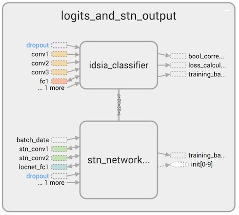
The STN converts the original images and feeds them to the IDSIA input, which is trained using backprop and then classifies the road signs.
Below is the part of the DAG, in which the original images are converted using STN and fed to the input of the classifier (IDSIA), which calculates the logits:
Now that we know the logit calculation method (STN + IDSIA network), the next step is to optimize the loss function (for which we will use cross-entropy or log loss — the standard choice for solving the classification problem):
Then we need to set operations (ops) for optimization and training, which should propagate errors back to the input layers:
I initialized a network with a high value of learning rate (0.02) so that gradients could more quickly spread information to the LocNet STN, which is located in the outer layers of the entire neural network. Otherwise, this network will learn more slowly (due to the problem of the “disappearing” gradient ). Small initial learning rate values do not allow neural networks to bring closer small road signs in the image.
The part of the DAG that calculates logits (network output) is added to the graph quite simply:
A piece of code above deploys the entire network - STN + IDSIA, we will discuss them in more detail below.
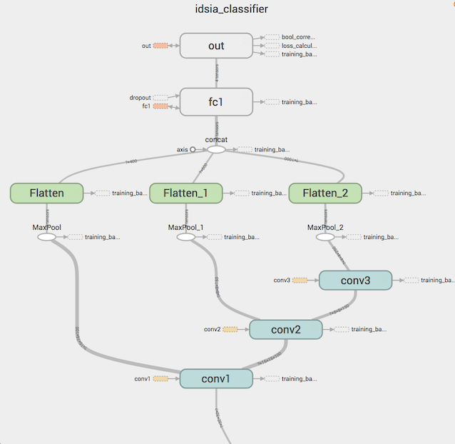
Inspired by the work of Moodstocks and the original article from the IDSIA Swiss AI Group, in which they used CNN to improve the previously achieved quality of the model, I took the general idea of the architecture of one network from the ensemble and implemented it in TensorFlow myself. The resulting structure of the classifier is as follows:
All this is illustrated below:
As can be seen, the results of the activation functions of each convolutional layer are combined into one vector, which is already served by fully connected layers. This is an example of multiscale-features that further improve the quality of the classifier.
The converted STN image is fed to the input of conv1 , as we discussed earlier.
Among the variety of models TensorFlow you can find the implementation of STN , which will be used in our network.
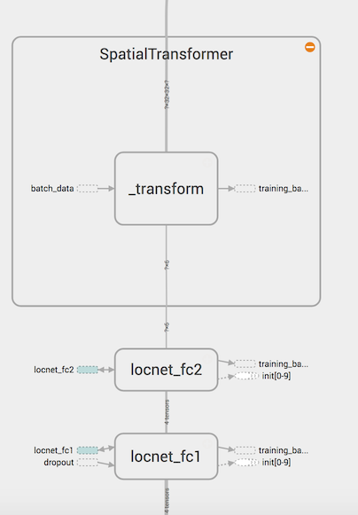
Our task is to identify and train LocNet, provide the transformer with the correct values of θ and insert the STN module into the DAG Tensorflow. The transformer generates a grid and provides transformation and interpolation.
The LocNet configuration is shown below:
LocNet convolutional layers:
Fully-connected part of LocNet:
The structure of convolutional layers LocNet is similar to IDSIA (although LocNet consists of 2 layers instead of 3, and in it we first do the pulling). More curious is the structure of fully connected layers:
The problem with using the STN module with CNN is the need to ensure that both networks are not retrained, which makes the learning process difficult and unstable. On the other hand, adding a small amount of augmented data (especially brightness augmentation) to a training set allows networks not to retrain. In any case, the advantages outweigh the disadvantages: even without augmentation, we get good results, and STN + IDSIA outperform IDSIA without this module by 0.5-1%.
In the process of learning the following parameters were used:
After 10 epochs, we get an accuracy of 99.3% on the validation data set. CNN is still being retrained, but do not forget that we use a double complex grid on the original dataset without its expansion by augmentation. In truth, by adding augmentation, I managed to get an accuracy of 99.6% on the validation set after 10 iterations (although the training time significantly increased).
Below are the model learning results ( idsia_1 is an IDSIA network without a module, idsia_stn is an STN + IDSIA). This is the accuracy of the entire network for validation.
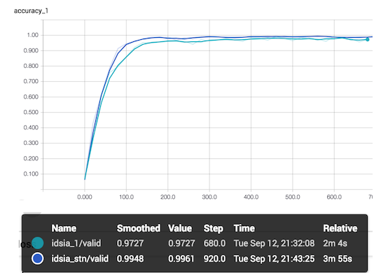
STN + IDSIA performs better than the IDSIA network without a module, although it takes longer to learn. I note that the accuracy in the graph above is calculated for the batch, and not for all validation.
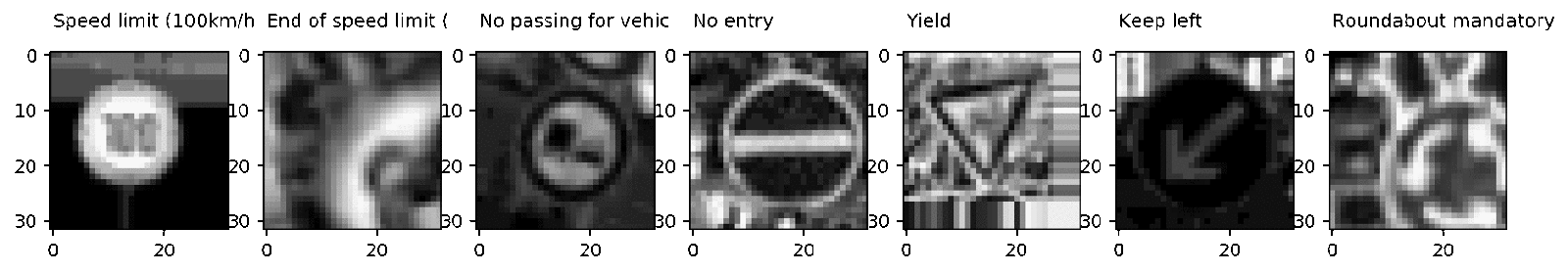
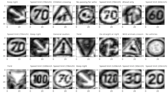
Finally, here is the result of the STN transformer after training:
Well, we summarize:
In the last post, we started talking about preparing data for training a convolutional network. Now is the time to use the data and try to build on them the neural network classifier of road signs. This is what we will do in this article, adding in addition to the classifier network a curious module - STN. Dataset we use the same as before .
Spatial Transformer Network (STN) is one of the examples of differentiable LEGO-modules, on the basis of which you can build and improve your neural network. STN, applying a learning affine transform followed by interpolation, deprives images of spatial invariance. Roughly speaking, the task of STN is to rotate or reduce-enlarge the original image so that the main classifier network can more easily determine the desired object. The STN block can be placed on a convolutional neural network (CNN), working for the most part on its own, learning from gradients coming from the main network.
')
All project source code is available on GitHub by reference . The original of this article can be viewed at Medium .
To have a basic understanding of how STN works, take a look at 2 examples below:
STN works even in difficult cases (for example, 2 characters in the image), but most importantly, STN really improves the quality of the classifier (IDSIA in my case).
Common STN device: young fighter course
One of the problems of convolutional neural networks is that the invariance to the input data is too low: different scale, point of shooting, background noise and much more . You can, of course, say that the pooling operation, so not favored by Hinton, gives some invariance, but in fact it simply reduces the size of the feature map, which results in the loss of information.
Unfortunately, due to the small receptive field in the standard 2x2 pooling, spatial invariance can only be achieved in deep layers close to the output layer. Also, pooling does not provide the invariance of rotation and scale. Kevin Zakka well explained the reason for this in his post .
The main and most common way to make the model resistant to these variations is dataset augmentation, which we did in the previous article :
Augmented images. In this post we will not use augmentation.
There is nothing wrong with this approach, but we would like to develop a smarter and more automated method for image preprocessing, which should help increase the accuracy of the classifier. Spatial transformer network (STN) - just what we need.
Below is another example of how STN works:
An example from the MNIST dataset from the original article. Cluttered MNIST (left), target, recognized STN (center), transformed image (right).
The work of the STN module can be reduced to the following process (not including training):
Application of STN conversion in 4 steps with a known matrix of linear transformations θ .
Now let's take a closer look at this process and each of its stages.
STN: conversion steps
Step 1. Determine the transformation matrix θ , which describes the transformation itself:
Affine transformation of the matrix θ .
Moreover, each transformation corresponds to its own matrix. We are interested in the following 4:
- Identical transformation (the output is the same image). These are our initial θ values. In this case, the matrix θ is diagonal:
theta = np.array([[1.0, 0, 0], [0, 1.0, 0]]) - Rotation (counterclockwise, 45º). cos (45º) = 1 / sqrt (2) ≈ 0.7:
theta = np.array([[0.7, -0.7, 0], [0.7, 0.7, 0]]) - Approaching . Approaching the center (2 times):
theta = np.array([[0.5, 0, 0], [0, 0.5, 0]]) - Distance Distance from the center (2 times):
theta = np.array([[2.0, 0, 0], [0, 2.0, 0]])
Step 2. Instead of applying the transform directly to the source image ( U ), create a sampling meshgrid of the same size as U. The sample grid is a set of indices (x_t, y_t) that cover the original image space. The grid does not contain any information about the color of the images. This is better explained in the code below:
# Implemented in https://github.com/tensorflow/models/blob/master/transformer/spatial_transformer.py # As I mentioned, we only need height and width of the original image def _meshgrid(height, width): with tf.variable_scope('_meshgrid'): x_t = tf.matmul(tf.ones(shape=tf.stack([height, 1])), tf.transpose(tf.expand_dims(tf.linspace(-1.0, 1.0, width), 1), [1, 0])) y_t = tf.matmul(tf.expand_dims(tf.linspace(-1.0, 1.0, height), 1), tf.ones(shape=tf.stack([1, width]))) x_t_flat = tf.reshape(x_t, (1, -1)) y_t_flat = tf.reshape(y_t, (1, -1)) ones = tf.ones_like(x_t_flat) grid = tf.concat(axis=0, values=[x_t_flat, y_t_flat, ones]) return grid Since this is the actual implementation in TensorFlow, in order to understand the general idea, we will translate this code into an analogue of numpy:
x_t, y_t = np.meshgrid(np.linspace(-1, 1, width), np.linspace(-1, 1, height)) Step 3. Apply a linear transformation matrix to the created sample grid to get a new set of points on the grid, each of which can be defined as the result of multiplying the matrix θ by the coordinate vector (x_t, y_t) with a free member:
Step 4. Obtain subsample V using the original feature map, transformed sample grid (see Step 3) and a differentiated interpolation function of your choice (for example, bilinear). Interpolation is necessary because we need to translate the result of the sampling (potentially possible fractional pixel values) into whole numbers.
Sampling and interpolation
The task of learning . Generally speaking, if we knew in advance the necessary θ values for each source image, we could begin the process described above. In fact, we would like to extract θ from the data using machine learning. This is quite realistic. First , we need to make sure that the loss function of the road sign classifier can be minimized using backprop through the sampler. Secondly , we find gradients in U and G (meshgrid): this is why the interpolation function must be differentiable or, at least, partially differentiable. Third , we calculate the partial derivatives of x and y with respect to θ . Technical calculations can be read in the original paper.
Finally, we create LocNet (a localizing network-regressor) , the only task of which is to train and predict the correct θ for the input image using the loss function, which was minimized through total backprop.
The main advantage of this approach is that we get a differentiable stand-alone module with memory (in the form of trained weights), which can be placed in any part of CNN.
Notice how θ changes as STN learns to recognize the target object (road sign) in the images.
Below is a diagram of the STN from the original article:
We reviewed all the steps involved in building an STN: the creation of LocNet, a sample mesh generator (meshgrid) and a sampler. Now we will build and train on TensorFlow the entire classifier, which includes in its graph and STN.
Build a model in TensorFlow
The entire model code, of course, does not fit into the framework of a single article, but it is available as a Jupyter laptop in the repository on GitHub .
In this article, I focus on some important parts of the code and the stages of learning the model.
First, our ultimate goal is to learn to recognize road signs, and to achieve it we need to create some kind of classifier and train it. We have many options: from LeNet to any other SOTA-neural network. In the process of working on the project, inspired by the work of Moodstocks on STN (implemented in Torch), I used the IDSIA neural network architecture, although nothing prevented me from taking something else.
At the second stage, we need to identify and train the STN module, which, taking the original image as input, converts it using a sampler and the output is a new image (or minibatch, if we work in batch mode), which in turn is used by the classifier.
I note that STN can be easily removed from the graph of calculations, replacing the entire module with a simple generator of batch. In this case, we just get the usual classifier network.
Here is the general scheme of operation of the obtained double neural network:
The STN converts the original images and feeds them to the IDSIA input, which is trained using backprop and then classifies the road signs.
Below is the part of the DAG, in which the original images are converted using STN and fed to the input of the classifier (IDSIA), which calculates the logits:
def stn_idsia_inference_type2(batch_x): with tf.name_scope('stn_network_t2'): # Unrolling the STN's LocNet -- stn_output is theta-matrix stn_output = stn_LocNet_type2(stn_convolve_pool_flatten_type2(batch_x)) # Grid generator and sampler transformed_batch_x = transformer(batch_x, stn_output, (32,32, TF_CONFIG['channels'])) with tf.name_scope('idsia_classifier'): # IDSIA uses transformed_batch_x from STN. Here we unroll the conv layers of IDSIA features, batch_act = idsia_convolve_pool_flatten(transformed_batch_x, multiscale=True) # Unrolling FC layers of IDSIA logits = idsia_fc_logits(features, multiscale=True) # Returning lots of objects. `logits` is the one that is really required for the model return logits, transformed_batch_x, batch_act Now that we know the logit calculation method (STN + IDSIA network), the next step is to optimize the loss function (for which we will use cross-entropy or log loss — the standard choice for solving the classification problem):
def calculate_loss(logits, one_hot_y): with tf.name_scope('Predictions'): predictions = tf.nn.softmax(logits) with tf.name_scope('Model'): cross_entropy = tf.nn.softmax_cross_entropy_with_logits(logits=logits, labels=one_hot_y) with tf.name_scope('Loss'): loss_operation = tf.reduce_mean(cross_entropy) return loss_operation Then we need to set operations (ops) for optimization and training, which should propagate errors back to the input layers:
boundaries = [100, 250, 500, 1000, 8000] values = [0.02, 0.01, 0.005, 0.003, 0.001, 0.0001] starter_learning_rate = 0.02 global_step = tf.Variable(0, trainable=False) learning_rate = tf.train.piecewise_constant(global_step, boundaries, values) with tf.name_scope('accuracy'): accuracy_operation = tf.reduce_mean(casted_corr_pred) with tf.name_scope('loss_calculation'): loss_operation = calculate_loss(logits, one_hot_y) with tf.name_scope('adam_optimizer'): optimizer = tf.train.AdamOptimizer(learning_rate=learning_rate) with tf.name_scope('training_backprop_operation'): training_operation = optimizer.minimize(loss_operation, global_step=global_step) I initialized a network with a high value of learning rate (0.02) so that gradients could more quickly spread information to the LocNet STN, which is located in the outer layers of the entire neural network. Otherwise, this network will learn more slowly (due to the problem of the “disappearing” gradient ). Small initial learning rate values do not allow neural networks to bring closer small road signs in the image.
The part of the DAG that calculates logits (network output) is added to the graph quite simply:
with tf.name_scope('batch_data'): x = tf.placeholder(tf.float32, (None, 32, 32, TF_CONFIG['channels']), name="InputData") y = tf.placeholder(tf.int32, (None), name="InputLabels") one_hot_y = tf.one_hot(y, n_classes, name='InputLabelsOneHot') #### INIT with tf.name_scope('logits_and_stn_output'): logits, stn_output, batch_act = stn_idsia_inference_type2(x) A piece of code above deploys the entire network - STN + IDSIA, we will discuss them in more detail below.
IDSIA: Classifier Network
Inspired by the work of Moodstocks and the original article from the IDSIA Swiss AI Group, in which they used CNN to improve the previously achieved quality of the model, I took the general idea of the architecture of one network from the ensemble and implemented it in TensorFlow myself. The resulting structure of the classifier is as follows:
- Layer 1: Convolutional (batch normalization, relu, dropout). Kernel : 7x7, 100 filters. At the entrance : 32x32x1 (In a set of 256). At the exit : 32x32x100.
- Layer 2: Max Pooling. To the entrance : 32x32x100. At the exit : 16x16x100.
- Layer 3: Convolutional (batch normalization, relu, dropout). Kernel : 5x5, 150 filters. At the entrance : 16x16x100 (in a batch of 256). At the exit : 16x16x150.
- Layer 4: Max Pooling. At the entrance : 16x16x150. At the exit : 8x8x150.
- Layer 5: Convolutional (batch normalization, relu, dropout). Kernel : 5x5, 250 filters. At the entrance : 16x16x100 (in a set of 256). At the exit : 16x16x150.
- Layer 6: Max Pooling. At the entrance : 8x8x250. Output : 4x4x250.
- Layer 7: Optional pooling for multiscale features. Kernels: 8, 4, 2 for layers 1, 2 and 3, respectively.
- Layer 8: Extending and concatenating features into a multiscale feature vector. At the entrance : 2x2x100; 2x2x150; 2x2x250. At the exit : feature vector 400 + 600 + 1000 = 2000 for fully connected layers
- Layer 9: Fully-connected (batch normalization, relu, dropout). At the entrance : 2000 signs (in a set of 256). 300 neurons.
- Layer 10: Logits (batch normalization). At the entrance : 300 signs. At the exit : logit (43 classes).
All this is illustrated below:
As can be seen, the results of the activation functions of each convolutional layer are combined into one vector, which is already served by fully connected layers. This is an example of multiscale-features that further improve the quality of the classifier.
The converted STN image is fed to the input of conv1 , as we discussed earlier.
Spatial Transformers in TensorFlow
Among the variety of models TensorFlow you can find the implementation of STN , which will be used in our network.
Our task is to identify and train LocNet, provide the transformer with the correct values of θ and insert the STN module into the DAG Tensorflow. The transformer generates a grid and provides transformation and interpolation.
The LocNet configuration is shown below:
LocNet convolutional layers:
- Layer 1: Max Pooling. At the entrance : 32x32x1. At the exit : 16x16x1.
- Layer 2: Convolutional (relu, batch normalization). Kernel : 5x5, 100 filters. Input : 16x16x1 (in a set of 256). At the exit : 16x16x100.
- Layer 3: Max Pooling. At the entrance : 16x16x100. At the exit : 8x8x100.
- Layer 4: Convolutional (batch normalization, relu). Kernel : 5x5, 200 filters. At the entrance : 8x8x100 (in a set of 256). At the exit : 8x8x200.
- Layer 5: Max Pooling. At the entrance : 8x8x200. At the exit : 4x4x200.
- Layer 6: Optional pooling for multiscale features. Kernels: 4, 2 for convolutional layers 1 and 2, respectively.
- Layer 7: Extruding and concatenating features into a vector . At the entrance : 2x2x100; 2x2x200. At the exit : vector of features with dimension 400 + 800 = 1200 for fully connected layers.
Fully-connected part of LocNet:
- Layer 8: Fully-connected (batch normalization, relu, dropout). At the entrance : 1200 signs (in a set of 256). 100 neurons.
- Layer 9: 2x3 matrix θ , which defines an affine transformation. Weights are given by zeros, the free term is a matrix similar to the unit one, with units on the main diagonal: [[1.0, 0, 0], [0, 1.0, 0]].
- Layer 10: Transformer: Grid generator and sampler implemented in spatial_transformer.py. This layer produces images with the same dimensions as the original (32x32x1), applying an affine transformation to them (thus, an approximate or rotated image is obtained).
The structure of convolutional layers LocNet is similar to IDSIA (although LocNet consists of 2 layers instead of 3, and in it we first do the pulling). More curious is the structure of fully connected layers:
Training and Results
The problem with using the STN module with CNN is the need to ensure that both networks are not retrained, which makes the learning process difficult and unstable. On the other hand, adding a small amount of augmented data (especially brightness augmentation) to a training set allows networks not to retrain. In any case, the advantages outweigh the disadvantages: even without augmentation, we get good results, and STN + IDSIA outperform IDSIA without this module by 0.5-1%.
In the process of learning the following parameters were used:
# TF Parameters TF_CONFIG = { 'epochs': 20, 'batch_size': 256, 'channels': 1 } # Omitting the model building phase (discussed earlier in this post) # ... # Train / validation datasets, see the previous post. # No augmentations. train_val_data = { 'X_train': X_tr_256, 'y_train': y_tr_256, 'X_valid': X_val_256, 'y_valid': y_val_256 } # Initializing the session and vars: sess = tf.InteractiveSession() sess.run(tf.global_variables_initializer()) # Skipping details and going to the training: for i in range(TF_CONFIG['epochs']): for batch_x, batch_y in batch_generator(train_val_data['X_train'], train_val_data['y_train'], batch_size=TF_CONFIG['batch_size']): _, loss, lr = sess.run([training_operation, loss_operation, learning_rate], feed_dict={x: batch_x, y: batch_y, dropout_conv: 1.0, dropout_loc: 0.9, dropout_fc1: 0.3} After 10 epochs, we get an accuracy of 99.3% on the validation data set. CNN is still being retrained, but do not forget that we use a double complex grid on the original dataset without its expansion by augmentation. In truth, by adding augmentation, I managed to get an accuracy of 99.6% on the validation set after 10 iterations (although the training time significantly increased).
Below are the model learning results ( idsia_1 is an IDSIA network without a module, idsia_stn is an STN + IDSIA). This is the accuracy of the entire network for validation.
STN + IDSIA performs better than the IDSIA network without a module, although it takes longer to learn. I note that the accuracy in the graph above is calculated for the batch, and not for all validation.
Finally, here is the result of the STN transformer after training:
Well, we summarize:
- STN is a differentiable module that can be integrated into a convolutional neural network. Standard use case is to place it immediately after the batch generator, so that it can train the transformation matrix θ , which minimizes the loss function of the main classifier (IDSIA in our case).
- The STN sampler applies an affine transformation to the source images (or feature map).
- STN can be considered as an alternative to image augmentation, which is a standard way to achieve spatial invariance for CNN.
- Adding one or more STN modules to CNN complicates learning, makes it unstable: now you need to make sure that both (instead of one) networks are not retrained. As it seems to me, this is one of the reasons why STN is not so common.
- STNs trained on augmented data (especially brightness augmentation) show better quality and do not retrain too much.
Source: https://habr.com/ru/post/339484/
All Articles