How the brain hits a tree, or how we made a recommendation system using a neural network.
How would you make a recommendation system? Many immediately had a picture in their head as they import and stack Xgboost CatBoost. Initially, the same picture appeared in our heads, but we decided to do this on neural networks in the HYIP wave, the benefit of which was a lot of time. The experience of their creation, testing, results and our thoughts are described below.
Formulation of the problem
We were faced with the task of creating a model that chooses people who should send an offer to use some service provided by the company. Previously, this was the decisive forest. We decided to do it on the “omnipotent” neural networks, at the same time understanding how they work and whether they are really complex. After studying the subject area, our attention focused on several architectures.
Interested in architecture
Further, by clicking on the name of something, you can get to the article, where it is well explained.
- CNN
The architecture used mainly for image processing.
What it is and how it works can be read here and here .
We decided to put it both separately and before LSTM for data compression and allocation of dependencies on transactions (which were presented in the form of very sparse tables).
By itself, it worked worse than when paired with LSTM, about which it is written further, but significantly accelerated training and improved quality.
We used convolutional networks with one-dimensional conv conv .
- Lstm
This is a popular architecture of the recurrent neural network, which showed itself well in the tasks of finding patterns on the time series, texts and classification, remembering important patterns, forgetting irrelevant ones.
Very detailed and understandable about its device is written here .
We used 2 LSTM layers in our task, each had 128 neurons.
Evaluated the work of three models based on the above architecture.
- This article provides a comparison of 3 networks, we took the one that showed the best result (FCN). The authors argue that this architecture is a good baseline for the classification of time series. In short, it consists of 3 blocks, in each of which first comes CNN-> BN ( batch normalization ) -> ReLU activation. After that comes the global average pooling.
- The architecture from this article . A typical approach to NLP is to represent words as a vector (embending), but the authors tried to encode the letters (using the one-hot encoding method), it turned out pretty good. We solved our problem in a similar way. Those. we have the words - these are categories, and the text is the history of the user's purchases. The architecture itself has the following form: (CNN-> MaxPooling) x3 -> Flatten -> (Dense-> Dropout) x2 -> Softmax.
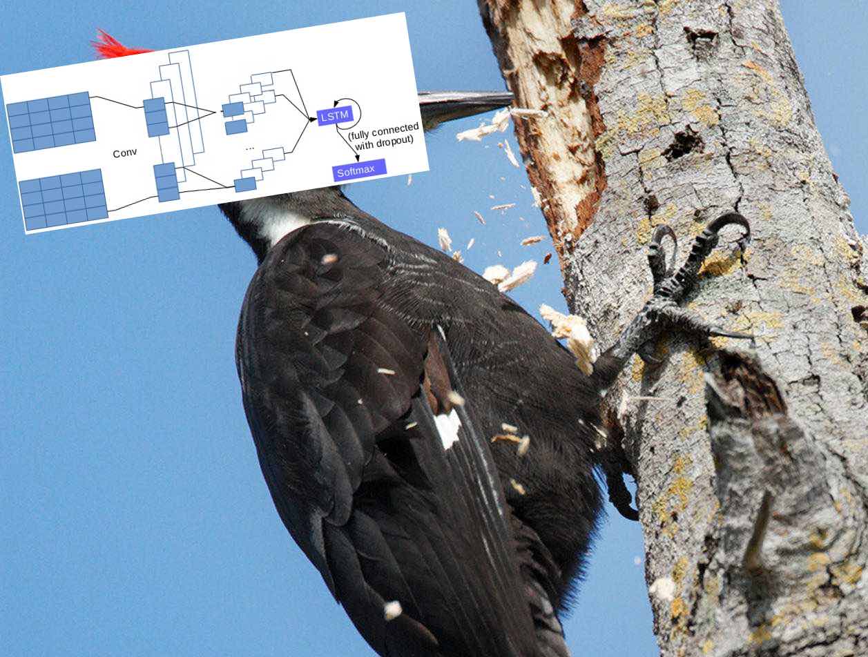
- After reading various blogs ( for example, this one ), I got the idea to try the following architecture: Conv1D-> Max Pooling-> LSTMx2 -> (Dense-> Dropout) x2-> Softmax.
Factorization
Imagine a matrix, each row is a user, each column is an item that the user can rate. The values of the matrix in position (i, j) are the estimate of the i-th user to the j-th item. Now, using the mathematical apparatus, we present this matrix as a product of two matrices (users, features) (features, objects). Where features are any signs that we highlight. Now, scalarly multiplying the user row by the subject column, we get a number indicating how much this subject likes this user.
Libraries for factoring:
lightfm
libfm- Pairwise
- Collaborative filtering is a prediction method based on the assumption that if people had similar behavior or ratings in the past, they would be similar in the future.
It can be based both on the external (explicit) behavior of users, when they themselves assess something (Netflix), and on implicit (regular) patterns, when their behavior coincides, in our case they have similar transactional sequences.
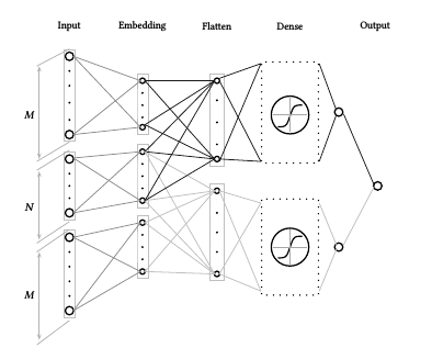
The approach of this article is based on collaborative filtering and takes into account both explicit and implicit regularities. The architecture is based on a neural network that examines user preferences by pairs of elements, taking into account the representations of these items, which were built before and stored in rows of matrices Us (user x feature), It (item x feature)
by analogy with matrix factorization. When training the network for the user, 2 subjects are selected for which he gave his estimates and the corresponding rows of the Us and It matrices are cut off, connected and served into the network. The loss function consists of two parts: the first is responsible for the losses at the output of the neural network itself, and the second is responsible for the fact that the scalar product of the vectors that were applied to the network training is also true. For example, we say that item_1 is better than item_2, which means that the neural network at the output should give a number greater than zero, and the scalar product of the corresponding vectors should be positive. Thus factoring is done using this neural network. Further, we assume that for each user there is a linear order on the items and based on this assumption we rank all the items for a specific user.
What did we do? We said that category_1 is better than category_2 if the user paid on it more often and based on this assumption they used this architecture.
A bit about data
QIWI provided us with a history of user purchases, as well as information that the user was recommended to buy, and whether he followed the recommendations within 15 days. We tried to predict the history of purchases of goods that he is likely to buy. We were interested in only a few categories of products (total of 5). Thus, we were able to measure the usual True True, False Positive, True Negative, False Negative and everything that depends on them for the categories we are interested in.
Also, the difficulty was that the data were greatly unbalanced, almost the entire volume of transactions lay in categories that we are not interested in.
Working process
Here we will discuss the behavior of models and the quality of various tests.
We will consistently describe how different models worked on different datasets.
Lstm
At the beginning we took a small amount of data, a transaction history of about 12k users and tried to predict the category of the next purchase. And this is how the above-mentioned architectures worked:
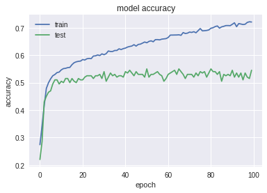
- Below is a schedule of working “bare” LSTM (LSTM-> Softmax). There were about 9 thousand users in the training, on the test - 3700 .
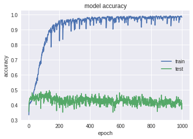
As you can see, she is very much retrained. The following quality metrics were obtained on the test data: Accuracy: 0.447; MRR: 0.576 . But having seen that it was pretty good soon, they thought that most likely our model predicts to the user what he basically bought. To do this, we checked the quality of the algorithm on those people whose predictable category is not present in the history of their transactions ( hereinafter referred to as special test ). There were not many such people in the test (approximately 500). They obtained the following results: Accuracy: 0.037; MRR: 0.205 . On such people, it quickly turned out noticeably worse.
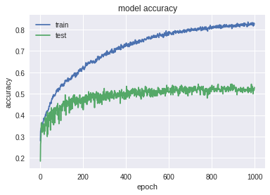
But we did not despair, tried various options with LSTM, eventually came to the following architecture: Conv1D-> Max Pooling-> LSTM (with rec dropout) x2 -> (Dense-> Dropout) x2-> Softmax. Here's how she worked:
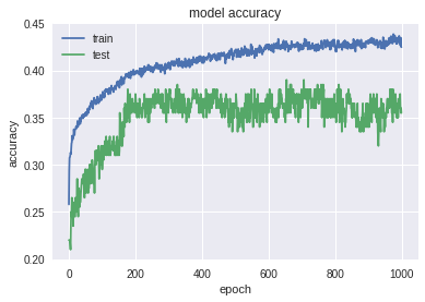
The picture is much better. The network is not so retrained. We look at the test soon : Accuracy: 0.391; MRR: 0.534 . The result is slightly worse than with the past network. But let's not rush to conclusions and look at the special test: Accuracy: 0.150; MRR: 0.312 . Thanks to a special test, we see that this model better finds patterns in the data. Remember this architecture, we still need it.
- Next, we evaluated the work of the following 2 architectures, which are based on CNN.
On the same data as in the previous paragraph, we launched FCN and Char CNN (their device was mentioned above). Learning outcomes:
The graph indicates retraining, but not as strong as with simple LSTM. The following results were obtained on the test: Accuracy: 0.529 MRR: 0.668 . On a special test: Accuracy: 0.014; MRR: 0.217 . Immediately look at the work of CNN's Char, but in fewer epochs:
Here the network is retrained much faster, it gives good results on the test, but according to a special test we see that it has poorly learned complex patterns:
Test: Accuracy: 0.543; MRR: 0.689 ;
Special test: Accuracy: 0.0098; MRR: 0.214 .
Pairwise
To begin with, we wrote our model according to the article.
We did this on Pytorch. This is a very convenient framework if you want to make an off-the-shelf neural network. Recently published an article with its description from mail.
First of all, we have achieved approximately the same quality of the NDCG as authors on dataset movielens .
After that we remade it for our data. We divided the data into two “temporary parts”.
At the entrance of the neural network, we gave a vector in which for each person for each category was the percentage of its payments to this category of the total. Therefore, the data were quite capacious, and she studied many times faster than LSTM, about 30 minutes on a video card, against several hours of LSTM.
Look at the quality.
At 300,000 users. Pomerin metrics for all classes, not just those that interest us.
| NDCG @ 5: 0.46 | Accuracy @ 3: 0.62 |
These indicators vary from sample (which users we take), changes within 7%.
Now a big datasset with several million users.
We study at all classes, and we rank only those that interest us.
The answer is considered correct if we predicted the class in which the user then paid.
The picture is approximately as follows:
| Class 1 (small) | Class 2 | Class 3 | Class 4 |
|---|---|---|---|
| almost doesn't predict it | the class is bigger, but she almost never predicts him | Precision = 0.45 Recall = 0.9 | Precision = 0.27 Recall = 0.6 |
Factoring (lightfm).
We used it for 500.000 users as well as in Pairwise, representing for each user for each category a percentage of payments to this category.
Everything can be seen from the training schedules (below is the iteration number).
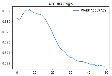

From the preceding paragraphs we can draw two conclusions:
- Our task is better solved by classification than ranking.
- A multi-class AUC is a specific thing and you should always look at how it counts.
results
After further testing, we decided that CNN + LSTM works better than others.
We took a big dataset and looked at how well the 5 classes we needed were predicted.
There were 5 million users on the training, 1.4 million users on the test. In order to increase the speed of learning (and it was necessary to increase it), we did not measure the intermediate quality of classification, so the training schedule will not be :(.
We are interested in conversion (precision). This metric shows the proportion of people who bought goods of this category, of the total number of people who were sent a recommendation of this category. It is clear that the good performance of this metric does not mean that the network works well, as it can recommend very little and achieve high conversion. Let's look at True Positive, False Positive, True Negative, False Negative to see the whole picture.
Below the table with 4 elements mean the following:
| True negative | False Positive |
|---|---|
| False negative | True positive |
Num - the number of people who actually belong to this class.
Class 1 :
| TN: 1440209 | FP: 1669 |
|---|---|
| FN: 3895 | TP: 1842 |
| precision | recall | f1-score | Num |
|---|---|---|---|
| 0.52 | 0.32 | 0.40 | 5737 |
Class 2 :
| TN: 1275939 | FP: 55822 |
|---|---|
| FN: 43994 | TP: 71860 |
| precision | recall | f1-score | Num |
|---|---|---|---|
| 0.56 | 0.62 | 0.59 | 115854 |
Class 3 :
| TN: 1136065 | FP: 108802 |
|---|---|
| FN: 91882 | TP: 110866 |
| precision | recall | f1-score | Num |
|---|---|---|---|
| 0.50 | 0.55 | 0.52 | 202748 |
Class 4 :
| TN: 1372454 | FP: 18812 |
|---|---|
| FN: 21889 | TP: 34460 |
| precision | recall | f1-score | Num |
|---|---|---|---|
| 0.65 | 0.61 | 0.63 | 56349 |
Class 5 :
| TN: 1371649 | FP: 18816 |
|---|---|
| FN: 22391 | TP: 34759 |
| precision | recall | f1-score | Num |
|---|---|---|---|
| 0.65 | 0.61 | 0.63 | 57150 |
Since we only look at 5 classes, we also need to add the class “other”, and, naturally, there are a lot more than the rest.
Class 6 (other) :
| TN: 18749 | FP: 327257 |
|---|---|
| FN: 2501 | TP: 1099108 |
| precision | recall | f1-score | Num |
|---|---|---|---|
| 0.77 | 1.00 | 0.87 | 1101609 |
Our network predicts very well the classes in which the user will pay in the next 15 days, even those that are several times smaller than others (for example, class 1 compared to the 3rd class).
Comparison with the previous algorithm.
Comparative tests on the same data showed that our algorithm provides several times greater conversion than the previous algorithm based on crucial forests.
Total
From our article we can draw several conclusions.
1) CNN and LSTM can be used for time series recommendations.
2) For a small number of classes it is better to solve the problem of classification, rather than ranking.
Neural networks is an interesting topic, but it takes a lot of time and can give unexpected surprises.
For example, our first Pairwise model on PyTorch worked poorly for the first week, because due to the abundance of code, somewhere in the error function, we cut off the distribution of the gradient.
Finally we introduce ourselves.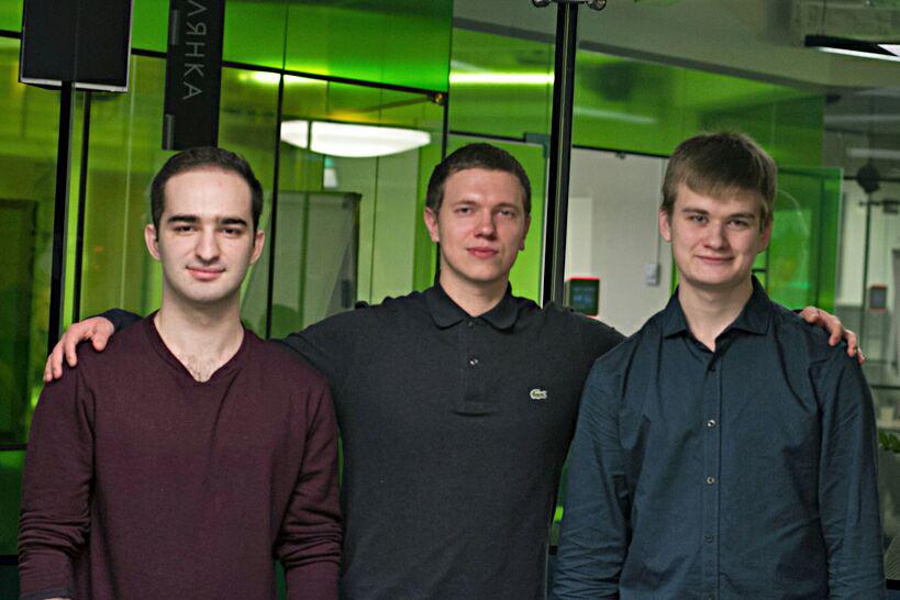
From left to right: Ahmedkhan ( @Ahan ), Nikolai, Ivan ( @VProv ). Ivan and Ahmedkhan are students of the Moscow Institute of Physics and Technology and underwent an internship, while Nikolai works at QIWI.
Thanks for attention!
')
Source: https://habr.com/ru/post/339454/
All Articles