Part 1. The calculation of the minimum number of moves to win using Markov chains

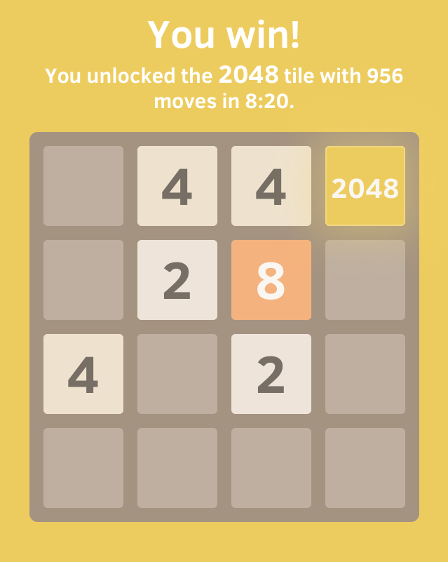
After a recent update, the “You win!” Screen of game 2048 began to show the number of moves required to win, and I wondered: how many moves are needed to win?

In the first part of the article, we will answer this question by simulating the 2048 game in the form of a Markov chain and analyzing it to show that, on average, no less than 938.8 moves are needed to win, on average . This gives us a good standard of reference - if you can win in about that number of moves, then you play well.

The number of moves needed to win depends on chance, because the game adds tiles 2 and 4 randomly. The analysis will also show that the distribution of the minimum number of moves to win has a standard deviation of 8.3 moves, and that its overall shape is well approximated by a mixture of binomial distributions.

To get these results, we will use the simplified version of 2048: instead of placing tiles on the field, we ... will throw them into the bag. That is, we will ignore the geometric constraints imposed by the shape of the field on which tiles can be combined. This simplification will greatly facilitate our work, because the player will no longer have to make any decisions ¹ , and because we will not need to track the position of tiles on the field.
')
The price of getting rid of these geometric constraints will be that we can only calculate the lower limit of the expected moves before the victory; it may happen that geometric constraints do not allow this boundary to be reached. However, having played many games in 2048 (for the sake of science!), I will also show you that in practice we can often get close to this border.

If you are unfamiliar with 2048 or with Markov's chains, then do not worry - I will explain the necessary concepts in the course of the article. The code (research quality), on the basis of which the article was written, is open source , in case you want to study the code for generating chains and graphs .

2048 as a chain of Markov

To present our simplified game “2048 in the bag” as a Markov chain, we need to specify the states and transition probabilities of the chain. Each state is something like a "cast" of the game at a certain point in time, and transition probabilities set the probability of transition to it for each state.

Here we will encode each state tiles that are currently in the bag. We do not care about the order of tiles, so we can perceive them as a set of tiles. Initially, there are no tiles in the bag, that is, the initial state is just an empty set. In the form of the diagram that we add below, this initial state looks like:

Field preparation

An example of a dozen fields for a new game.

When we start a new game in 2048, the game has two random tiles on the field (see examples above). To represent this in a Markov chain, we need to specify transition probabilities from the initial state to each of the possible subsequent states.

Fortunately, we can look at the source code of the game to see how the game does it. When a game places a random tile on the field, it always follows this scenario: selects a cell at random, then adds a new tile, either with a value of 2 (with a probability of 0.9) or with a value of 4 (with a probability of 0.1) .

In the case of “2048 in a bag,” we are not worried about finding a free cell, because we did not put any restrictions on the capacity of the bag. We are only interested in adding tile 2 or 4 with a given probability. This leads to three possible subsequent states from the initial state:

• $$$\ left \ {2,2 \ right \}$ when both new tiles have a value of 2 . It happens with probability $$$0.9 \ times 0.9 = $ 0.8$ .
• $$$\ left \ {4,4 \ right \}$ when both new tiles have a value of 4 . It happens with probability $$$0.1 \ times 0.1 = 0.01$ , that is, you are quite lucky if you start the game with two fours.
• $$$\ left \ {2,4 \ right \}$ when new tiles have a value of 2 , and then 4 , what happens with the probability $$$0.9 \ times 0.1 = 0.09$ , or first 4 , and then 2 , what happens to the probability $$$0.1 \ times 0.9 = $ 0.0$ . We do not care about the order, so both cases lead to the same state with a common probability $$$0.09 + 0.09 = 0.18$ .

We can add these subsequent states and their transition probabilities to the Markov chain scheme as follows (transition probabilities are written on the edges, and new nodes and edges are marked in blue):

Playing a game

Having placed the first pair of tiles, we are ready to start the game. In a real game, this would mean that the player needs to be held left, right, up or down to connect pairs of identical tiles. However, in our game with the bag, nothing prevents us from connecting all pairs of identical tiles, so we will do it.

The rule of combining tiles in a game with a bag will be as follows: we find in the bag all pairs of tiles that have the same value, and delete them; then replace each pair of tiles with one tile with double value of ² .

After combining pairs of identical tiles to go to the next state, the game randomly adds one new tile, using the process already described above, that is, tile 2 with probability 0.9 or tile 4 with probability 0.1.

For example, to find possible subsequent state states $$$\ left \ {2,2 \ right \}$ , we first combine two tiles 2 into one tile 4 , and then the game adds either tile 2 or tile 4 . Thus, possible subsequent states will be $$$\ left \ {2,4 \ right \}$ and $$$\ left \ {4,4 \ right \}$ which, as it happens, we met earlier. Then the circuit containing these two transitions from $$$\ left \ {2,2 \ right \}$ which have a probability of 0.9 and 0.1, respectively, will be:



If we continue this process for subsequent states $$$\ left \ {2,4 \ right \}$ , then we will see that while the union is impossible, because there are no pairs of identical tiles, and the subsequent state will be either $$$\ left \ {2,2,4 \ right \}$ or $$$\ left \ {2,4,4 \ right \}$ , depending on whether the new tile has a value of 2 or 4 . Then the updated scheme will be like this:

Layers and “passes”

We can continue to add transitions in this way. However, with the addition of new states and transitions, the schemes can become more complex ³ . We can streamline the schemes a bit using the following observation: the sum of tiles in the bag increases with each transition either by 2 or 4 . This is because combining pairs of identical tiles does not change the sum of the values ​​of the tiles in the bag (or on the field - this property applies to the real game), which means that the game adds Tile 2 or Tile 4 .

If we group the states by their sum into “layers”, the first few layers will look something like this:


To reduce the noisiness of the schemes, for later layers, I also do not indicate the marks for transitions with a probability of 0.9 (solid lines if they are not marked in any way) and 0.1 (dotted lines).

When grouping states into layers by sums, one more regularity becomes apparent: each transition (except transition from the initial state) takes place either to the next layer with a probability of 0.9, or into the layer after it with a probability of 0.1. (This is especially obvious if you look at the layers with the amounts of 8, 10 and 12 from the diagram above.) That is, the game most often gives us 2 , and we move to the next layer, but sometimes we are lucky and the game gives us 4 , and this means that we can skip a layer, which brings us a little closer to our goal - reaching tile 2048.

End of the game

We can continue this process forever, but since we are only interested in the achievement of tile 2048 , we will stop it at this moment, making any state with tile 2048 absorbing . The absorbing state has a single transition that leads to itself with a probability of 1. That is, having reached the absorbing state, it will no longer be able to get out of it.

In this case, all absorbing states are “states of victory” - we received Tile 2048 , which means we won the game. In the "game with the bag" there is no possibility to "lose", because unlike the real game, we cannot get into a situation when the field (or bag) is filled.

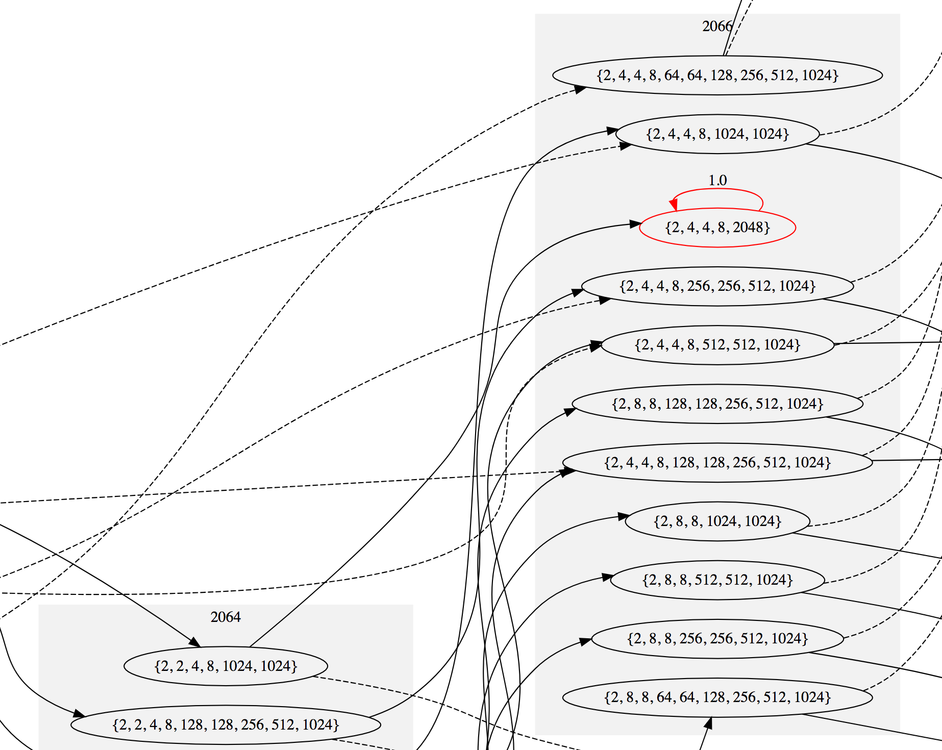
The first state containing Tile 2048 is in a layer with a sum of 2066. It is noteworthy that it is impossible to get a single Tile 2048 on the field - to combine tiles 1024 , tiles 512 , and so on, several moves are required for which more tiles 2 and 4 accumulate. Therefore, the sum of tiles for the first state with tile 2048 higher than 2048.

Here is what the graph looks like near this first winning state ( see details ). Absorbing states are highlighted in red:



If we continue to add transitions until there are no nonabsorbing states, then we end up with 3487 states, 26 of which are absorbing; this completes the definition of a Markov chain. The scheme of the complete circuit is quite large, but if your computer is able to cope with the 5-megabyte SVG file, then here is the complete circuit diagram (you may have to scroll down a little to see the beginning). If you zoom out, it will look like this:

Chain samples

Now that we have invested so much effort in modeling the 2048 game (in the bag) in the form of a Markov chain, we need to figure out how many moves are required to achieve all the absorbing states. The easiest way to do this is to run simulations. In each simulation, we will generate one trajectory along the chain, starting from the initial state, then choosing the next state randomly, in proportion to the transition probabilities, and then repeating the process from this state. After performing one million simulations for the number of moves before the victory, the following distribution is revealed:



The average, marked with a vertical blue line, is equal to 938.8 strokes , excluding the first transition from the initial state, with a standard deviation of 8.3 strokes . So, here is our answer to the question of the minimum expected number of moves before winning the game!

Markov chain theory also allows us to compute some of these properties directly, using clever mathematics. In Appendix A, I will show how to calculate the average number and standard deviation for the number of moves without using a simulation. Then, in Appendix B, I will use some of the properties of the chain to offer at least a partial explanation of the shape of the distribution curve.

We check theory with practice

Finally, to test these results in real life, I played many times in 2048 (for the sake of science!) And in 28 games won, I recorded the number of moves and the amount of tiles on the field when I reached tile 2048 ⁴ :



Writing these numbers to a spreadsheet and plotting them, I got the following scatter diagram:



I marked in blue the minimum expected number of moves, plus or minus one standard deviation, and in red the amount of tiles 2066, which, as we found out, is the minimum amount of tiles possible if there is a tile in 2048.

The sum of tiles on the field is important, because if it is large, then this usually means that I made a mistake and drove a large tile somewhere, from where I cannot combine it with another tile. Then it took much more moves to re-build this tile on the spot from where it can be merged (or to change the field configuration to move it to the right place to merge) with another large tile.

If I played well in 2048, we could predict that my results would be grouped in the lower left corner of the chart, and that most of them would lie between the dotted blue lines. In fact, as we see, even though sometimes I come up to the ideal, the result is not very stable - quite a lot of points in the upper right corner with a bunch of extra moves and tiles.

This chart also highlights the fact that our analysis gives us only the minimum expected number of moves. There were several games in which I was lucky and I won in less than 938.8 moves, including a victory with 927 moves and a total of 2076 tiles. (This is the second left result in the bottom row of the compilation.) This happened because I accidentally lost a lot of 4 tiles 4 game, and also because I didn’t make serious mistakes that required extra moves.

In principle, there is a non-zero probability that we can win the game in just 519 moves. We can determine this by passing along the chain, always choosing the transition towards 4 and counting the number of transitions needed to reach the 2048 tile. However, the probability of such an outcome is equal to $$$0.1 ^ {521}$ , or $$$10 ^ {- 521}$ . In the universe we observe, there are only about $$$10 ^ {80}$ atoms, so it is not necessary, with bated breath, to wait that such a game will fall out just for you. Also, if we are very unlucky and we will always get tiles 2 , we can still win in just 1032 moves. Such a game is much more likely, its probability is equal $$$0.9 ^ {1034}$ which is approximately equal to $$$10 ^ {- 48}$ , so, most likely, and this game should not wait, with bated breath. The average of 938.8 moves is much closer to 1032 than 519, because the probability of the appearance of tiles 2 much higher than that of tiles 4 .

Conclusion

In this part, we have considered a method of creating a Markov chain, which simulates the evolution of the game of 2048 in the case when the union of identical tiles is always possible. Thanks to this, we were able to apply the techniques of the Markov absorbing chains theory to calculate the interesting properties of the game, and, in particular, we found out that, on average, at least 938.8 moves are required to win.

The main simplification that allowed us to use this approach is to ignore the field structure. That is, we assumed that we were throwing tiles into the bag, and not placing them on the field. In the second part, I plan to consider the case when we take into account the structure of the field. We learn that the number of states that need to be considered becomes many orders of magnitude larger (although perhaps not as much as one might think), and realize that we have to leave the world of Markov chains, going into the world of Markov decision-making processes which will allow us to return to the player’s equations. In principle, we will be able to completely "solve" the game, that is, to find, perhaps, the best way to play.

Appendix A: Markov Chain Analysis

After setting the Markov chain, we can attract the power of mathematics to perform calculations of its properties without simulation. Many of these calculations are possible only because our Markov chain belongs to a special kind of Markov chain, called the Markov absorbing chain .

To treat absorbing chains, the Markov chain must meet the following criteria:

1. It must have at least one absorbing state. As we saw above, in our chain there are 26 absorbing states, one for each winning state with a tile of 2048 .
2. Any state can reach an absorbing state in a finite number of transitions. One way to determine this is to make sure that there are no other cycles in the chain except for the absorbing states: with the exception of the absorbing states, the chain is a directed acyclic graph.

Transition matrix

Now that we have determined that we have an absorbing Markov chain, the next step is to write its transition matrix in the canonical form . The transition matrix is ​​a matrix that orders the transition probabilities, which for our chain we have defined above, such that $$$(i, j)$ is the transition probability $$$i$ in state $$$j$ .

To transition matrix $$$\ mathbf {P}$ absorption chain with $$$r$ absorbing states and $$$t$ non-returnable (i.e. non-absorbing) states could be in canonical form, it should be possible to break it into four smaller matrices $$$\ mathbf {Q}$ , $$$\ mathbf {R}$ , $$$\ mathbf {0}$ and $$$\ mathbf {I}$ such that:

$$

$$\ mathbf {P} = \ left (\ begin {array} {cc} \ mathbf {Q} & \ mathbf {R} \\\ \ mathbf {0} & \ mathbf {I} _r \ end {array} \ right)$$

Where $$$\ mathbf {Q}$ Is a matrix $$$t \ times t$ describing the probability of transition from one non-return state to another non-return state, $$$\ mathbf {R}$ Is a matrix $$$t \ times r$ describing the probability of transition from a non-returnable state to an absorbing state, $$$\ mathbf {0}$ denotes a matrix $$$r \ times t$ zeros and $$$\ mathbf {I} _r$ - is a transition matrix for absorbing states, which is the unit matrix $$$r \ times r$ .

In order to transform the transition matrix of our chain into a canonical form, we need to determine the order of states. It will be sufficient to order the states (1) according to whether they are absorbing (absorbing states go last), then (2) by the sum of their tiles (in ascending order) and, finally, (3) in lexical order to get rid of dependencies. If we do this, we get the following matrix:



It is quite large, namely, the size $$$3487 \ times 3487$ , therefore, when zooming out, it looks almost diagonal, but if we bring the lower right corner closer, we will see that it has a structure, and, in particular, a canonical view, to which we aspire:

Fundamental matrix

Having obtained the canonical form of the transition matrix, then we use it to find what is called the fundamental matrix of the chain. It allows us to calculate the expected number of transitions before absorption, that is, we (finally!) Will find the answer to our original question.

Fundamental matrix $$$\ mathbf {N}$ is set relatively $$$\ mathbf {Q}$ identical equality

$$

$$\ mathbf {N} = \ sum_ {k = 0} ^ {\ infty} \ mathbf {Q} ^ k \ mathbf {N} = \ sum_ {k = 0} ^ {\ infty} \ mathbf {Q} ^ k$$

Where $$$\ mathbf {Q} ^ k$ denotes $$$k$ -th degree of the matrix $$$\ mathbf {Q}$ .

Element $$$(i, j)$$$ m a t h b f N has a certain interpretation: this is the expected number of times we will enter the state$\ mathbf {N}$$$j , if we follow the chain starting from the state$j$$$$i$ . To see this, we can notice that as an element $$$(i, j)$ matrices $$Q is the transition probability$\mathbf{Q}$$$i in state$i$$$j in one transition, and the element$j$$$$(i, j)$ matrices $$Q k is the probability of entering the state$\mathbf{Q}^k$$$j exactly for$j$$$k transitions after entering the state$k$$$$i$ . If for a given pair of states $$$i$ and $$j we summarize the mentioned probabilities for all$j$$$k ≥ 0 , then the sum will include each time we have the opportunity to enter the state$k \geq 0$$$j after condition$j$$$i , weighted by the appropriate probability, which gives us the desired expectation. Fortunately, the fundamental matrix can be calculated directly, without unpleasantly infinite summation, as the inverse matrix$i$

$$$\mathbf{I}_t - \mathbf{Q}$ where $$I t is the identity matrix.$\mathbf{I}_t$$$$t \times t$ . I.e, $$$\mathbf{N} = (\mathbf{I}_t - \mathbf{Q})^{-1}$ . (Proof of this will be homework for the reader!)

Expected number of moves to win

Having obtained a fundamental matrix, we can find the expected number of transitions from any state $$i to the absorbing state by summing all the elements in the row$i$$$i - in other words, the number of transitions before entering the absorbing state is equal to the total number of transitions that we had to perform in all non-return states along the way. We can get these sums of series at once for all states by calculating the product of the matrix by the vector$i$

$$$\mathbf{N} \mathbf{1}$ where $$1 denotes a column vector$\mathbf{1}$$$$t$ . Insofar as $$N = ( I t - Q ) - 1 , we can do this by solving a linear system of equations$\mathbf{N} = (\mathbf{I}_t - \mathbf{Q})^{-1}$

$$

$$(\mathbf{I}_t - \mathbf{Q})\mathbf{t} = \mathbf{1}$$

for $$$\mathbf{t}$ . Element in $$t , corresponding to the initial state (empty set$\mathbf{t}$$${ } ) is the number of transitions. In this case, the resulting number is 939.8. To complete, we only need to subtract$\left \{ \right \}$$$1 , because the transition from the initial state is not considered a move. This gives us the final answer -938.8 moves. We can also get the variance for the minimum number of moves as$1$

$$

$$2(\mathbf{N} - \mathbf{I}_t) \mathbf{t} - \mathbf{t} \circ \mathbf{t}$$

Where $$∘ stands for the(component) Hadamard product. For the initial state, we obtain a variance of 69.5, which gives us a standard deviation of8.3 steps.$\circ$

Appendix B: distribution curve shape

It is noteworthy that we were able to calculate both the mean and the variance of the distribution of moves before the victory from the Markov chain using the fundamental matrix. However, it would be nice to know why the distribution turned out this form. The approach I suggest here is only approximate. but it closely matches the empirical results from the simulation and gives us some useful information.

We will start with a return to the observation made earlier: the sum of tiles on the field increases with each transition by 2 or 4 (except for the first transition from the initial state). As we will see below, if we were interested in getting a specific amount on the field, rather than getting a tile 2048, then it would be quite easy to calculate the necessary number of transitions using a binomial distribution.

So, the next question will be how much we want to receive. From the above analysis of the Markov chain, we determined that there are 26 absorbing (winning) states. We also saw that they are on different “layers of sums,” that is, there is not one sum to which we aspire, there are several of them. We need to know what is the probability for each state to become absorbed. It is called the probability of absorption . Then we can sum up the absorption probabilities for each of the absorbing states in a separate layer of sums in order to find the probability of winning with a particular resulting sum.

Absorption probability

Fortunately, the absorption probabilities can also be found from the fundamental matrix. In particular, we can obtain them by solving linear equations

$$

$$(\mathbf{I}_t - \mathbf{Q}) \mathbf{B} = \mathbf{R}$$

for matrix $$ m a t h b f B size$\ mathbf {B}$$$t × r whose element$t \times r$$$( i , j ) is the probability of absorption in the state$(i, j)$$$j starting at the state$j$$$$i$ .As before, we are interested in the probabilities of absorption, when starting from the initial state. Having built the graph of the absorption probability, we will see that there are 15 absorbing states, the probabilities of which are large enough to be displayed on the graph (no less than$$$10^{-3}$ ):



In particular, most games end with either state $${ 2 , 2 , 8 , 8 , 2048 } , the amount of which is equal to 2068, or the state$\left \{ 2,2,8,8,2048 \right \}$$${ 2 , 4 , 16 , 2048 } , the sum of which is 2070. Summing up all the absorbing states by the sum of the layers, we get the total probabilities of the sum of the layer:$\left \{2,4,16,2048\right \}$

Binomial probabilities

Now, when we have amounts that can be targeted, and we know how often we aim at each, the next question is: how many moves do you need to get a specific amount? As noted above, we can perceive this question as applied to the binomial distribution , which allows us to calculate the probability of a given number of “successes” from a given number of “attempts”.

In this case, by “attempt” we will mean a move, and by “success” - a move in which the game gives us a tile 4; as shown above, this happens with a probability of 0.1. The “failure” here is the move in which the game gives us a tile 2, which happens with a probability of 0.9.

Given this interpretation of success, in order to get a given amount$$$S$ behind $$M moves, we need$M$$$S2 -Msuccesses of$\frac{S}{2} - M$$$M moves. So it turns out, because each move adds to the sum at least$M$$$2 , which generally gives$2$$$2 M , and each success adds to the amount of additional$2M$$$2 , making in general$2$$$$2 \left(\frac{S}{2} - M\right) = S - 2M$ . By adding these values, we get the desired amount $$$S$ .

Then the joint probability of receiving the sum $$S for the number of moves$S$$$M is binomial, and in particular$M$

$$

$$\mathrm{Pr}(M=m, S=s) = B\left(\frac{s}{2} - m; m, 0.1\right)$$

Where $$B ( k ; n , p ) is the mass distribution function for the binomial distribution, which gives us the probability of getting exactly$B(k; n, p)$$$k success for$k$$$n attempts where the success rate is equal$n$$$$p$ i.e.

$$

$$B(k; n, p) = {n\choose k}p^k(1-p)^{n-k}$$

Where $$( nk )denotes thebinomial coefficient. Now that we know the target amount$n \choose k$

$$S , to which we strive, we can calculate the conditional distribution of moves, taking into account that the amount that interests us is from the joint distribution. That is, we can find$S$$$$\mathrm{Pr}(M | S)$ as

$$

$$\mathrm{Pr}(M | S) = \frac{\mathrm{Pr}(M, S)}{\mathrm{Pr}(S)}$$

Where $$P r ( S ) is obtained from the joint distribution by summation$\mathrm{Pr}(S)$$$M for each possible amount$M$$$$S$ . It is worth noting that $$P ( S ) is less than one for each possible amount, because there is always a chance that the game will “skip” the amount by issuing us a tile. Having obtained all these conditional distributions for each target amount, we can add them, weighted by the total probability of absorption for the target amount, to get the overall probability. This gives us a fairly exact match with the distribution from the simulation:$\mathrm{P}(S)$4





Here, the simulated distribution is shown in gray columns, and each of the conditional distributions is shown in colored areas. Each conditional distribution is scaled according to the total absorption probability for its sum, and also shifted by several moves, because larger sums on average require more moves.

One of the interpretations of this result: in an optimal game, the number of moves before a win depends strongly on how quickly a player can get an amount large enough to contain a 2048 tile, which in turn depends on the number of tiles 4following the binomial distribution.

---

Thanks to Hope Thomas and Nate Stemen for editing the drafts of this article.

Notes

1. , , . .
2. : , 2 , , , 4 , 8 .
3. dot graphviz . dot , .
4. The appearance of the “You win!” Screen over the months of collecting this data has changed several times. For the record: all these months, I not only played in 2048.

Part 2. Counting states using combinatorics

In the previous part, I found out that an average of at least 938.8 moves is required to win a 2048 game . The main simplification that allowed us to perform these calculations was that we ignored the structure of the field - in essence, we threw tiles into the bag, rather than placing them on the field. Thanks to this bag-based simplification, we were able to simulate the game in the form of a Markov chain with only 3486 states.

In this part we will make the first attempt to count the number of states without simplification with the “bag”. That is, in this part of the statewill contain the complete field configuration, defining the tiles present in each cell of the field. Therefore, it is worth expecting that there will be much more states of this type, because they include the positions of tiles (and cells without tiles). As we will see, that is exactly the case.

To do this, we will use (simple) techniques from enumerated combinatorics to exclude some states that can be written but which cannot occur in the game, for example, as mentioned above. The results will also be applicable to all games similar to 2048, even to fields played (and not just 4x4) and to other tiles (not only to2048). We will see that such games in smaller fields and / or to tiles of smaller importance have much fewer states than the full game of 4x4 in 2048, and that the techniques used here are relatively much more effective in reducing the expected amount of condition with a small field size. As a bonus, we will also see that the 4x4 field is the smallest square field on which it is possible to reach the tile 2048.

The code (research quality) on which this part is based is open source , in case you want to evaluate the implementation or code for the graphs .

Baseline

The most obvious way to estimate the number of states of the game 2048 is the following observation: there are 16 cells, each cell can be empty or contain a tile, the value of which is one of 11 powers of two, from 2 to 2048. This gives us 12 possible values ​​for each of 16 cells, that is just $$12 16 , or 184 quadrillion (approximately$12^{16}$$$10 17 ) possible values ​​that can be written in this way. For comparison:according to some estimates, the number of possible configurations of positions on a chessboard is approximately equal to$10^{17}$$$10 45 , andaccording to the latest estimates, in go$10^{45}$$$10 170 states, so at least$10^{170}$$$10 17 is a lot, but it is not a record for games. In a more general form, such 2048 games can be represented as follows:$10^{17}$

$$B - the size of the field, and$B$$$K - the degree of the winning tile with the value$K$$$$2^K$ . For convenience, let $$C denotes the number of cells per field, i.e.$C$$$$C=B^2$ . For a typical 2048 game with a 4x4 field: $$$B=4$ , $$C = 16 , and$C=16$$$K = 11 because$K = 11$$$2 11 = 2048 , and the possible number of states is$2^{11} = 2048$

$$

$$(K + 1)^C$$

Now let's see how we can clarify the possible value.

First, because the game ends when we get the tile$$2 K , then we do not care where this tile is and what is on the field besides it. Therefore we can combine all states with tile$2^K$$$2 K in one special state of "victory." In the remaining states, each cell can be either empty or contain one of the tiles.$2^K$$$$K - 1$ . This reduces the number of states that interest us to

$$

$$K^C + 1$$

Where $$1 is a state of "victory." Secondly, we can observe that some of these states$1$

$$K C can never occur in a game. In particular, the rules of the game imply two useful properties:Property 1:there are always at least two tiles on the field.Property 2:there is always at least one tileor tileon the field.The first property is observed, because even if you start the game with two tiles and combine them, you will still have one, after which the game will add one random tile and there will be two of them. The second property is observed because the game always adds a tileor a tileafter each turn.Thus, we know that in any valid state there must be at least two tiles on the field, and one of them must be tileor tile$K^C$



24

24

24. To accommodate this, we can subtract all states without a tile 2or without a tile 4, which$$( K - 2 ) C , as well as states with only one tileand the remaining empty cells, which$(K-2)^C$2$$C , as well as states with only one tileand other empty cells, which are also$C$4$$$C$ . This gives us a possible meaning.

$$

$$K^C - (K-2)^C - 2C + 1$$

states. Of course, when$$$K$ or $$C is great, it almost looks like$C$$$K C , that is, the primary term, but for small values ​​this adjustment is more significant. Let's use this formula to reduce the possible number of states for different size fields and maximum tiles:$K^C$

Maximum Tile	Field size
	2x2	3x3	4x4
eight	73	19,665	43 046,689
sixteen	233	261,615	4,294,901,729
32	537	1 933 425	152 544 843 873
64	1,033	9,815,535	2 816 814 940 129
128	1,769	38 400 465	33,080,342,678,945
256	2,793	124,140,015	278 653 866 803 169
512	4,153	347,066,865	1 819 787 258 282 209
1024	5,897	865 782 255	9 718 525 023 289 313
2048	8,073	1,970,527,185	44,096,709,674,720,289

You can immediately see that in games with 2x2 and 3x3 fields there are many orders of magnitude fewer states than in a 4x4 game. In addition, we managed to limit the possible number of tiles in a 4x4 game to 2048 "only" by 44 quadrillions, or ~$$$10^{16}$ .

To deal with these numbers of states a little more, we can use another important property, which was useful in the previous part:

Property 3: the sum of tiles on the field increases with each move by 2 or 4.

This rule is observed, because the union of two tiles does not change the amount of tiles on the field, and after it the game adds 2or 4.

Property 3 implies that the states during the game never repeat. This means that we can order states into layers according to the sum of their tiles. If the game is in a state with a layer of 10, we know that the next state will be in a layer with a sum of either 12 or 14. It turns out that we can also count the number of states in each layer.

Let be $$S denotes the sum of tiles on the field. We want to count the number of ways that$S$$$C numbers, each of which is a power of two from 2 to$C$$$2 K - 1 , can be folded to get$2^{K-1}$$$$S$ .

Fortunately, this turns out to be a kind of well-studied combinatorial problem: counting the compositions of an integer . In general, the composition of an integer$$S is an ordered collection of integers, which together give$S$$$$S$ ;each integer in the aggregate is called a part . For example, for an integer$$3 there are four compositions, namely$3$$$$1 + 1 + 1$ , $$$1 + 2$ , $$$2 + 1$ and $$$3$ .When there are restrictions for parts, for example, to be a power of two and the presence of a certain number of parts, then such a composition is called limited .

Even more fortunate, Chinn and Niederhausen (2004) ¹ have already studied just this type of limited composition and derived recursion, which will allow us to count the number of compositions that have a certain number of parts, each part being a power of two. Let be $$N ( s , c ) denotes the number of (positive) whole compositions.$N(s, c)$$$s exactly in$s$$$c parts, and each part is a power of two.$c$ Then

$$

$$N(s, c) = \begin{cases} \sum_{i = 0}^{\lfloor \log_2 s \rfloor} N(s - 2^i, c - 1), & 2 \le c \le s \\\ 1, & c = 1 \textrm{, } s \textrm{ - 2} \\\ 0, & \textrm{ } \end{cases}$$

because for each composition number $$$s - 2^i$ at $$c - 1 parts we can get the composition$c - 1$$$$s$ of $$c parts, adding one part with the value$c$$$$2^i$ .

Now we need to make small changes to the limits of summation: we need to use the powers of two, starting from 2 and $$2 K - 1 , because if we have a tile$2^{K-1}$$$2 K , then the game is won. For this let$2^K$$$N m ( s , c ) denotes the number of compositions of the number$N_m(s, c)$$$s exactly in$s$$$c parts, with each part being a power of two from$c$$$$2^m$ before $$$2^{K-1}$ . According to the above logic, this can be given by the equation

$$

$$N_m(s, c) = \begin{cases} \sum_{i = m}^{K - 1} N(s - 2^i, c - 1), & 2 \le c \le s \\\ 1, & c = 1 \textrm{, } s = 2^i \textrm{ } i \in \{ m, \ldots, K-1 \} \\\ 0, & \textrm{ } \end{cases}$$

Now we have a formula for exactly $$c parts, but we need a formula for the parts to be up to$c$$$$c$ . You can use the same reasoning as in the previous section: subtract the states without tiles 2 or 4, which are $$$N_3(s, c)$ . According to property 1, we need at least two parts, so we begin to summarize with $$$c=2$ . This gives us as a possible value for the number of states with the sum $$$s$

$$

$$\sum_{c = 2}^{C} {C \choose c} \left( N_1(s, c) - N_3(s, c) \right)$$

Here $$( Cc )is abinomial coefficientgiving us a number of ways to choose$C \choose c$$$c of possible$c$$$C cells in which tiles are placed. Let's mark them on the chart.$C$


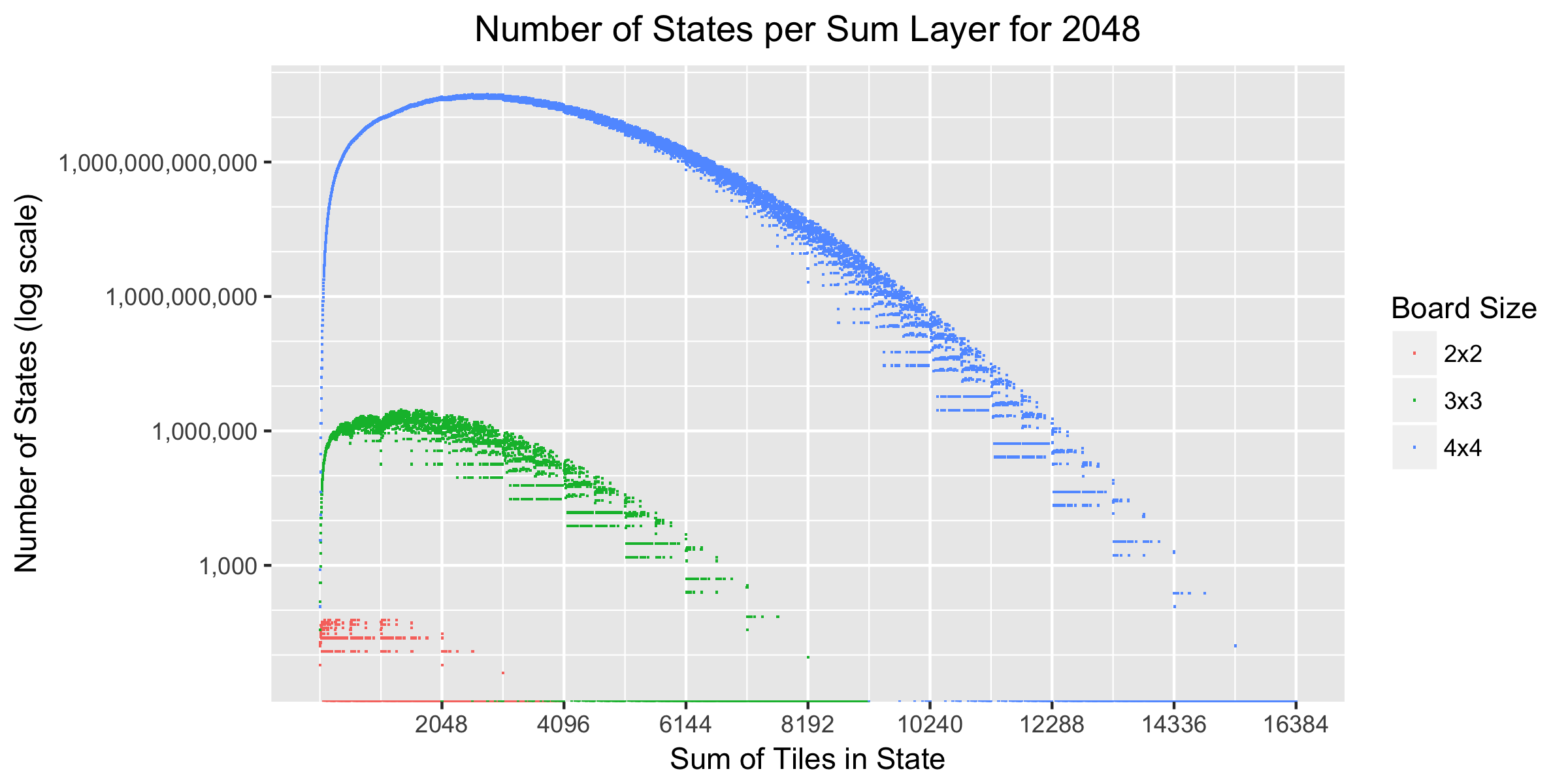
Regarding order, we can see that a 2x2 game never has more than 60 states per layer, a 3x3 game has a maximum of about 3 million states per layer, and a 4x4 game has a maximum of about 32 trillion ( $$10 13 ) states per layer. The number of states is growing rapidly in the early stages of the game, but then it slows down and gradually decreases when the field is filled. On the declining part of the curve, we see gaps, especially for large amounts. This can happen when there are no tiles that fit the field and are added to this value. The upper limit on the horizontal axis arises because we may have$10^{13}$

$$C values ​​each up to$C$$$2 K - 1 , that is, the maximum attainable amount is$2^{K-1}$$$C 2 K - 1 , or 16 384 for a game 4x4 to 2048.Finally, it is worth noting that if we add the number of states in each layer across all possible sums of layers from 4 to$C 2^{K-1}$

$$C 2 K - 1 and we add one for the singular state of the gain, then we get the same number of states that was expected in the previous section. This is a useful check on the correctness of our reasoning.$C 2^{K-1}$

Layer reachability

Another useful consequence of property 3 is that if two consecutive layers do not have states, then later layers cannot be achieved. This is because the amount can increase by a maximum of 4 per turn; if there are two adjacent layers with no states, then the sum should increase by 6 in one turn in order to “jump over” to the next layer, which is impossible. Thus, finding the sums of layers that do not contain states with the help of the above calculations allows us to narrow the possible value by excluding the states in the unreachable layers after the last reachable layer. Maximum achievable layer sums (without unreachable tile 2048):

Field size	Maximum attainable layer total
2x2	60
3x3	2,044
4x4	9 212

This table also shows us that the maximum tile we can reach on a 2x2 field is a tile 32, because a tile 64cannot appear in a layer with a sum of 60 or less. Similarly, the maximum reachable tile on a 3x3 field is a tile 1024. This means that a 4x4 field is the minimum square field on which tile 2048 ² can be reached . In the case of a 4x4 field, the maximum amount of the layer that can be reached without reaching the tile 2048(that is, without winning) is 9,212, but if you allow the tile 2048, you can also achieve greater amounts.

Given the reachability of the layers, the new possible values ​​for the number of states will be:

Maximum Tile	The way	Field size
		2x2	3x3	4x4
eight	Baseline	73	19,665	43,046,689
	Layer reachability	73	19,665	43,046,689
sixteen	Baseline	233	261,615	4,294,901,729
	Layer reachability	233	261,615	4,294,901,729
32	Baseline	537	1 933 425	152 544 843 873
	Layer reachability	529	1 933 407	152 544 843 841
64		1 033	9 815 535	2 816 814 940 129
		905	9 814 437	2 816 814 934 817
128		1 769	38 400 465	33 080 342 678 945
		905	38 369 571	33 080 342 314 753
256		2 793	124 140 015	278 653 866 803 169
		905	123 560 373	278 653 849 430 401
512		4 153	347 066 865	1 819 787 258 282 209
		905	339 166 485	1 819 786 604 950 209
1024		5 897	865 782 255	9 718 525 023 289 313
		905	786 513 819	9 718 504 608 259 073
2048		8 073	1 970 527 185	44 096 709 674 720 289
		905	1 400 665 575	44 096 167 159 459 777

This greatly affects the 2x2 field, reducing the number of states from 8,073 to 905 for the game to 2048, and it is noteworthy that the values ​​for the number of reachable states do not increase from 905 for the maximum tiles after 32, because on the 2x2 field it is impossible to reach tiles larger than 32. It also has a slight effect on the 3x3 field, but on 4x4 it has a relatively small impact - we get rid of “only” about 500 billion states of the total number in the case of a game before 2048.

In graphical form, these data look like this:

Conclusion

We obtained approximate estimates of the number of states in game 2048 and in similar games on smaller boards and smaller maximum tiles. So far, our best estimate of the number of states in a 4x4 game to 2048 is approximately 44 quadrillion (~$$$10^{16}$ ).

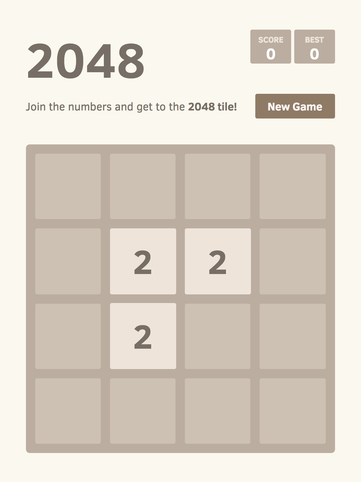
It is likely that this and other assessments are greatly exaggerated, because for many reasons, conditions that are unattainable in the game can be taken into account. For example, the state from the illustration to the title of this part of the article:


satisfies all the constraints we considered, but in the game it is still impossible to achieve it: to get into it, we would have to move the tiles in some direction, and we would move two tiles 2to the edge of the field. Perhaps there is a way to fine-tune the above calculation arguments taking this into account (and, most likely, to other restrictions), but so far I have not figured out how to do this!

In the next post, we will see that the number of really attainable states is much lower, in fact listing them. There will still be a lot of them for the 3x3 and 4x4 fields, so we will need knowledge of the theory of information processing, as well as mathematics.

---

If you've read this far, you might want to follow me on Twitter , or even send a request for hire to Overleaf .

Notes

1. Chinn, P. and Niederhausen, H., 2004. Compositions into powers of 2. Congressus Numerantium , 168, p.215. ()
2. , , , 2048 . , , . , , , 4x4 131072 ( $$$2^{17}$ ), . — , , . , - , 8192 , « » 131072